Practical 2 Estimation and descriptive statistics
Our goal in science is to understand properties of populations. We want to know things like: how big is the average blue whale? And we want to test questions, such as: are whales in the Pacific Ocean bigger than whales in the Indian Ocean?
The challenge is that we cannot measure every single individual (or thing), we have to take a smaller "sample" from the population and measure "statistics" on this sample. When we call a statistic an "estimate", we mean that it represents some number that we have not measured directly. When we have an estimate of something, we also need to know how good that estimate is. Intuitively, if we take a sample of five blue whales and calculate the sample mean (average) body mass, we will not be very confident that this sample average (based on only five individuals) represents the average body mass of all blue whales in the ocean.
In this practical you will:
- Be introduced to some experimental data that you will use in this prac and the next;
- Calculate various "descriptive statistics" (estimated properties of populations);
- Learn how to write your own function to calculate a statistic;
- Learn how to do perform calculations on a single sample of one population and on samples from different populations;
- Learn how to utilise simulations of data to explore the idea of "standard error", and how it relates to "standard deviation".
- Begin to learn how to address the question: "how can one judge the relative merits of separate studies that address the same question"?
2.1 The cure for cancer
Two research teams were both awarded $1M in funding to investigate the potential of several drugs to cure cancer. Both teams claim to have discovered a new drug, "Cureallaria", which is a cure for all cancers (as well as acne, hair loss, and yellow teeth!).
Below are the data collected by each research team, separated into control (no Cureallaria) and treatment (Cureallaria) groups. Each datum is the proportion of a group of 100 people that were cancer-free after being given either the treatment or the control.
Research Team "A"
Research team A used their preliminary $1M in funding to replicate the initial 200 person (100 control + 100 treatment) study as many times as possible. They were able to repeat their study 10 times.
Research Team "B"
Research team B were so impressed with the massive difference between their treatment and controls in the first round of experiments that they only replicated the experiment three times (for 100 control and 100 treatment individuals each time). Encouraged by these early findings, Team B spent the rest of the initial $1M of funding on advertising and media releases, telling the world about their incredible results, and preparing their business structures for massive cash inflows.
Based on these results, both Research Teams are requesting $10M million in further funding to develop their cures into a product for commercial distribution across the entire world. As the adviser to the Minister for Science you must present a summary of each research team's data so that she can decide which of the team will receive the funding, and which will miss out.
2.2 Calculating descriptive statistics
Go into the CONS7008 R Project folder on your computer and click on the "CONS7008 R Project.Rproj" file (depending on your computer you may not see the ".Rproj" file extension). RStudio should open automatically (it might take a little while, be patient). In RStudio, go to File -> New File -> R Script and a blank R script will appear. Now press File -> Save. Rename the file "Prac 2 R script.R" and save it inside the "R scripts" folder. For today's prac, paste your scripts into this R script and run the commands from there (remember to save the script at the end of the session!).
The "Cureallaria" data already exists as a csv file in the "Data" subfolder within your R Project. We can read it in and explore it like this:
## read in the data and call it "cancer_data"
cancer_data<-read.csv("Data/Cureallaria.csv", stringsAsFactors = TRUE) ## using "stringsAsFactors = TRUE" forces R to convert character variables to factors (it is useful most of the time)

## look at the first six rows
head(cancer_data)

## look at a summary of the data
summary(cancer_data) ## this is very informative!


## look at a plot of the data - this is a box and whisker plot

par(mfrow=c(1,2))## set up a plotting canvas with 1 row and two columns

## plot Team A
with(subset(cancer_data, Team == "A"), plot(N_cured_from_100 ~ Treatment, main = "Team A"))

## plot Team B
with(subset(cancer_data, Team == "B"), plot(N_cured_from_100 ~ Treatment, main = "Team B"))

## close the plotting device and reset plotting parameters
dev.off()
2.3 Measures of "central tendency"
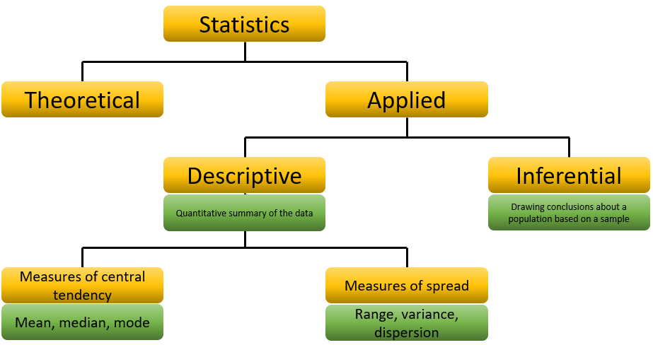
"Central tendency" is the most basic property that a data sample can have. Common measures of central tendency are mean and median, both alternative ways to locate the "middle" of the data.
With your tutor and peers, discuss what "central tendency" might mean. How would you measure it?
The tendency of data to be "close to" or "clump around" a particular value.
2.3.1 Calculting the mean and median
Run the code below to use the built-in R function for calculating the mean (called mean!) to obtain the mean of each of the samples. Because the data is in "tidy" format (i.e. long format, more on "tidy" data later), we need to separate the data into each combination of Team and Treatment. There are many ways to do this but here we use "subset".
NB: if you put () around a line of code, the output will be stored AND appear in the console!
subset_A_Control<-subset(cancer_data, Team=="A" & Treatment=="Control")
mean(subset_A_Control$N_cured_from_100)

subset_A_Cureallaria<-subset(cancer_data, Team=="A" & Treatment=="Cureallaria")
mean(subset_A_Cureallaria$N_cured_from_100)

subset_B_Control<-subset(cancer_data, Team=="B" & Treatment=="Control")
mean(subset_B_Control$N_cured_from_100)

subset_B_Cureallaria<-subset(cancer_data, Team=="B" & Treatment=="Cureallaria")
mean(subset_B_Cureallaria$N_cured_from_100)
You now have four means, one for each of the team's control and treatment groups.
Which of the 4 means is highest?
Team B "Cureallaria"
Repeat what you did above, but calculate the median instead of the mean, again using the in-built R function.
Are either of these "central tendency" statistics enough to judge which team deserves the funding?
No; they all ignore the spread (scatter) within the data sample and the sample size! We will be less confident that our sample mean represents the actual population mean if it was calculated on a sample of five highly variable numbers than if it was calculated on a sample of 300 numbers with lower spread.
2.4 Measures of "spread"
Along with measuring the "middle" of a data sample, it is also important to measure the "spread" of a data sample around this centre. How far are the data values from the middle value? There are several measures of spread that we can calculate from our sample to "estimate" the spread of data in the population. We will use built-in functions in R to calculate these. You can check your lecture notes to refresh your memory of the formula for these summary statistics if you are interested.
sd(subset_A_Control$N_cured_from_100) ## Standard deviation, or "SD"
var(subset_A_Control$N_cured_from_100) ## Variance (SD squared)
range(subset_A_Control$N_cured_from_100) ## Range, simply the minimum and maximum value
Duplicate and edit the code to repeat these commands for Team B.
Should spread be measured in the same units as the raw data?
Not necessarily. The standard deviation is, however, in the same units as the raw data. Thus, for variables with a larger mean, the SD will also be larger.
2.5 Calculating summary statistics across an entire data set
Above, we calculated summary statistics for each subset of the data. However, because our data are "tidy" (i.e., in long format), we can use shortcuts! One such shortcut is the "aggregate" function. Here we can calculate the mean of each combination of Team and Treatment in a single line of code!
## the aggregate function is SUPER handy for summarising information for different combinations of groups (here we use Team and Treatment as the groups)
aggregate(N_cured_from_100 ~ Team + Treatment, data = cancer_data, FUN = mean)
Now, instead of using mean as the function, try other functions, such as: FUN = var, FUN = sum, FUN = min, FUN = length. What do they do?
Based on all of the summary statistics you have calculated so far, which Research Team should the minister fund? Why?
We'll come back to this question in the Practical 3!
What benefit can you think of for Team A having conducted 10 experiments of 200 individuals each versus one big experiment with 1,000 people?
The expected mean values of each small versus one big experiment are the same, but we can estimate the uncertainty by having many small experiments.
2.6 Writing your own functions
While the base package (i.e., R itself) and other publicly available packages come with loads of useful functions (like mean and var), anyone can write an R function.
Below is an example of how you might create your own mean function.
The mean (\(\bar{x}\)) of a set of numbers is their sum (\(\sum x_i\)) divided by the number of samples (\(n\)):
\(\bar{x} = \frac{\sum x_i}{n}\)
We can use built-in functions to calculate sum(x) and length(x) (assuming "x" is a vector of numbers).
Run this code, but remember that when you see a "{" you must submit ALL the code up to and including the closing parenthesis "}" - otherwise you leave R hanging - waiting on you to finish the command!:
myMean <- function(x){       ## Define the function and its input; an arbitrary set of numbers ('x')
  Total <- sum(x)            ## Sum the elements of 'x' and store as 'Total'
  SampleSize <- length(x)    ## Count how many elements there are in 'x'
  Mean <- Total/SampleSize   ## Calculate the mean of 'x' by dividing the sum by the number of samples
  return(Mean)               ## Tell R what to 'spit out'
}                            ## End the definition of the function
The function, myMean, is now part of the "R armoury"; you created it! If you look over in the top right panel of your RStudio and scroll down, you will see a "Functions" sub-panel, and myMean listed there.
You can now use myMean in the same way as any other function:
NB: any function you define disappears when you end your session.
Here is an example of something useful that is not built in: A function to calculate another metric of central tendency of data, the "mode". This is simply the value within the data that occurs most frequently:
mode <- function(x){                               ## Name the function ('mode') and its input: an arbitrary vector ('x')
  x_table<-table(x) ## use the handy "table" function to calculate how many times each value is represented
  as.numeric(names(which(x_table==max(x_table)))) ## extract the value(s) that are most numerous
}                                               ## End function definition
Having defined it, you can now apply that function to calculate the mode of any set of numbers.
mode(subset_A_Control$N_cured_from_100) ## Use the function to calculate the mode of 'subset_A_Control'
Why does mode return ten values for "subset_A_Control"?
All of the values are unique! None are represented more than once!
What are the relative advantages of mean, median, and mode as statistics describing "central tendency?
You could talk all day about this! Here's a question to get you started:
What happens to each if you have a large outlier, e.g. c(2, 1.9, 2.1, 2, 2.3, 1000)?
2.7 Simulating data based on "population" parameters
The Australian Bureau of Statistics (ABS) reported that Australian's aged 18-44 years old have an average height of 1.704 m (SD = 0.066). Height is a normally (Gaussian) distributed variable. Height is a useful variable to think about because the frequency distribution is very well characterised. Indeed, human height is one of those rare variables where the number of observations in our measurement space might approach the total number of individuals in our population, or sample space.
Let's first simulate our "population"; At the time, the ABS reported ~6 million people in our focal age group (18-44 yo). We can simulate a data sample that will mimic the true distribution of height using the R command rnorm. This function simulates a normal distribution of our liking and takes random draws from it. It is possible to simulate distributions of other kinds in R too - we will examine these other types of distributions later in the course. For now, let's simulate our normal distribution with a mean of 1.704 and a standard deviation of 0.066:
## Simulate 6,000,000 data points with mean = 1.704 and sd = 0.066
SimData <- rnorm(n = 6000000, mean = 1.704, sd = 0.066)
Now, let's treat this simulated distribution as the TRUE population distribution (i.e., let's pretend that we actually measured all 6 million people ourselves!). We can now explore how taking different samples from a population influences our understanding of the population from which we sampled, and particularly our understanding of the "true" central value and spread of height.
Conveniently, R has a function called sample that takes random samples from a variable. Copy and run this code to take a sample of 10 individuals from our population (called "SimData"):
## "sample" 10 objects from that population, making sure to sample any object only once (replace = FALSE)
SimData10 <- sample(SimData, 10, replace = FALSE)
SimData10 ## Look at the heights of your 10 sampled individuals

## Calculate basic, descriptive statistics
mean(SimData10)
sd(SimData10)
Did your sample accurately represent the population?
You probably answered "no" to this question - we expect that any random sample of a population might not reflect the actual values of that population, and this is particularly true when our sample is small
When you call the sample function (or the rnorm function), you get a different set of numbers each time. Therefore, if you re-run the code above, you will get slightly different means and standard deviations for each sample. Give it a go.
Start a new chunk of code to record your estimates. You should create two new objects, one for Means and one for SampleSize - use the c() function to concatenate the data for each. For example, I took five different samples of 10 individuals and estimated the mean of each:
Means <- c(1.7275, 1.6854, 1.8012, 1.7101, 1.6833)
SampleSize <- c(10, 10, 10, 10, 10)
Now do the same, and then take samples for a few larger samples sizes (e.g., 100, 1000, 10000). To be clear, repeat what you did for a sample size of 10, but now use samples sizes of 100, 1000, 10000.
Hint: your "SampleSize" vector should look like this (five of each sample size):
SampleSize <- c(10, 10, 10, 10, 10, 100, 100, 100, 100, 100, 1000, 1000, 1000, 1000, 1000, 10000, 10000, 10000, 10000, 10000)
Your "Means" vector will have the same number of values (20 values).
Once you have taken all samples and calculated the 20 means, plot them against sample size:
Each object within the "Means" vector is a sample mean. Is mean(Means) close to 1.704?
As the number of sample means increases, the distribution of sample means approximates a normal (Gaussian) distribution with the mean approximately equal to the mean of the population, \(\mu\), from which the samples were taken.
What is this property of a set of sample means?
CENTRAL LIMIT THEOREM!
Now let R do the work of storing the means:
Ns <- c(10, 100, 1000, 10000)  ## Sample sizes for R to work with
Nreps <- 50 ## Number of reps per sample size (i.e. number of sample means calculated per sample size. Above we used 5, but we can use 50 here)

Results <- matrix(nrow = Nreps, ncol = length(Ns)) ## Set up a blank matrix to store results
colnames(Results) <- Ns

## this is called a "for loop" - we will explain!!!
for(i in 1:length(Ns)){  ## For each sample size
  for(k in 1:Nreps){     ## For each replicate
    Results[k, i] <- mean(sample(SimData, Ns[i], replace = FALSE))  ## Record the sample mean in the kth row based on the ith sample size
  }
}

Results  ## Look at the results
Each "sample" provides an "estimate" of the population mean (in this case, we know that the true mean is 1.704); the sample means are stored in "Results".
NB: we could have done exactly the same for the standard deviation - each "sample" provides an estimate of the true population standard deviation of 0.066.
Now, let's plot the results. We need the data in a slightly different format (which requires the "tidyverse" package; you may need to install.packages("tidyverse")):
library(tidyverse)  ## Load the library
## use the wonderful "pivot_longer" function
ResultsLong<-pivot_longer(as.data.frame(Results), everything(), names_to = "SampleSize", values_to = "SampleMean", names_transform = as.numeric)

## now plot the results
with(ResultsLong, plot(SampleMean ~ jitter(SampleSize, 0.5), col = SampleSize))  ## Plot the sample means by the sample sizes
abline(h = 1.704)  ## Add the true population mean
NB: the jitter(SampSize, 0.5) jitters the values around the x-axis a little bit - otherwise all the points would fall on top of one another.
What do you notice about the estimates for the three different sample sizes?
They are ALL fairly close to the 1.704!
The sample means with n = 10000 are always very close to mean = 1.704.
The sample means with n = 10 bounce around a lot more, but are fairly close to mean = 1.704.
If you didn't know the mean and standard deviation of this "population", in which "estimate" of the mean would you be most confident? Hopefully the one with more samples - it is clearly more accurate!
Again: the distribution of sample means approximates a normal (Gaussian) distribution with the mean approximately equal to the mean of the population. We can plot this property...
The following code adds Gaussian density lines to the plots you have just seen (we also flip the x- and y-axes because it's just a little bit easier to visualise). Don't worry too much about what the code is doing, just think about what it produces:
## Prepare the density plots
D10 <- density(Results[, 1], adjust = 2)
D100 <- density(Results[, 2], adjust = 2)
D1000 <- density(Results[, 3], adjust = 2)

## Scale the density plots so that they are visible
D10$y <- D10$y * 2 + 10
D100$y <- D100$y * 2 + 100
D1000$y <- D1000$y * 2 + 1000

## now make the plot
with(ResultsLong, plot(SampleMean, SampleSize, col = SampleSize,
                       ylim = c(0, max(D1000$y)),
                       xlim = c(min(D10$x), max(D10$x))))
abline(v = 1.704)
lines(D10, col = 10)
lines(D100, col = 100)
lines(D1000, col = 1000)
You should see from these density plots that they approximate a normal distribution. The peaks of the distributions sit approximately on the population mean (Central Limit Theorem!!!), and the curve is a lot flatter for 10 samples compared to 85 samples.
2.8 Standard error of the mean
The "standard error" quantifies the "level of uncertainty", or accuracy, of an "estimate" (e.g., the "estimated" population mean). The standard error of the mean can be thought of like this: it is the spread of possible values for the true population mean. It is related to the standard deviation, which measures the spread of the data itself, but it is not the same thing. The standard error is calculated by dividing the sample standard deviation by the sqrt of the sample size (referred to as "n").
The figure in the previous section showed that that "spread" was large when the sample size was 10, but small when the sample size was 10000.
Let's demonstrate this by sampling from our height data:
SimData10 <- sample(SimData, 10, replace = FALSE)     ## Sample 10 individuals
SimData100 <- sample(SimData, 100, replace = FALSE)   ## Sample 100 individuals
SimData1000 <- sample(SimData, 1000, replace = FALSE) ## Sample 1000 individuals

sd(SimData10)   ## Calculate the standard deviation for SimData10
sd(SimData100)  ## Calculate the standard deviation for SimData100
sd(SimData1000) ## Calculate the standard deviation for SimData10000

## The standard error is calculated as follows (there is no inbuilt function):
sd(SimData10)/sqrt(length(SimData10))     ## Calculate the standard error for SimData10
sd(SimData100)/sqrt(length(SimData100))   ## Calculate the standard error for SimData100
sd(SimData1000)/sqrt(length(SimData1000)) ## Calculate the standard error for SimData10000
What happened to the standard deviation as the number of samples increased?
Not much hopefully! Remember that the sample standard deviation is simply an "estimate" of the true standard deviation of the population (although it should become more accurate with more samples).
What happened to the standard error as the number of samples increased?
The standard error decreased!
As you obtain more samples, you become more confident that the "sample" mean is close to the "population" mean. The range of "possible" population mean values decreases.
What is the difference between standard error and standard deviation?
Standard deviation simply describes the spread of the data.
Standard error describes your confidence in an estimate.
We will come back to this idea in the next practical, and use it to test questions such as, "which research team should we fund"?
2.9 List of useful functions
Here are a few useful functions that you learned today.
Measures of central tendency
mean; median
Measures of spread
sd; var
Other descriptive statistics
max; min; range; length; quantile
Apply functions to groups
aggregate
Binding by column and row
cbind; rbind
Convert objects
tidyverse::pivot_longer
Sampling
sample; rnorm