Practical 7 Linear mixed-effects models (LLMs)
One of the fundamental assumptions of statistical models is that each observation is independent. That means we can build a model that relies on each data point equally to estimate model parameters (i.e., intercepts and slopes). But a lot of times in ecology and conservation science, we've collected data that are NOT independent. By not independent, we mean that values of response variables are likely to be similar based on some kind of underlying correlation, usually created by grouping. This grouping could be data from the same subregion (from the online module), replicates of experiments in the same block or tank, or repeated measures studies where the same animals (but preferably plants) are re-measured over time. We'll cover examples of each of these in this prac to give you a gentle introduction (as gentle as this stuff can be...).
The core advance in mixed-effects models is to associate non-independent data together, telling the model they can't be relied on as independent. Instead they have an association that needs to be accounted for in the model. We do this via "random effects". This turns the model from "complete pooling" (all the data are in one big pool) to "partial pooling" (each group of related data have their own pool, but we can make generalisations across the pools). Mixed-effects models estimate overall (i.e. population-level) intercepts and slopes, just like we expect from simpler models, but they also give us separate intercepts (and slopes if required) for each group of observations, capturing the variation in our response variable that is attributable to the grouping.
This prac will explore three examples of data that should be modelled via mixed-effects models.
7.1 Simple nested data
Climate predictors of Sandhill Dunnart fitness
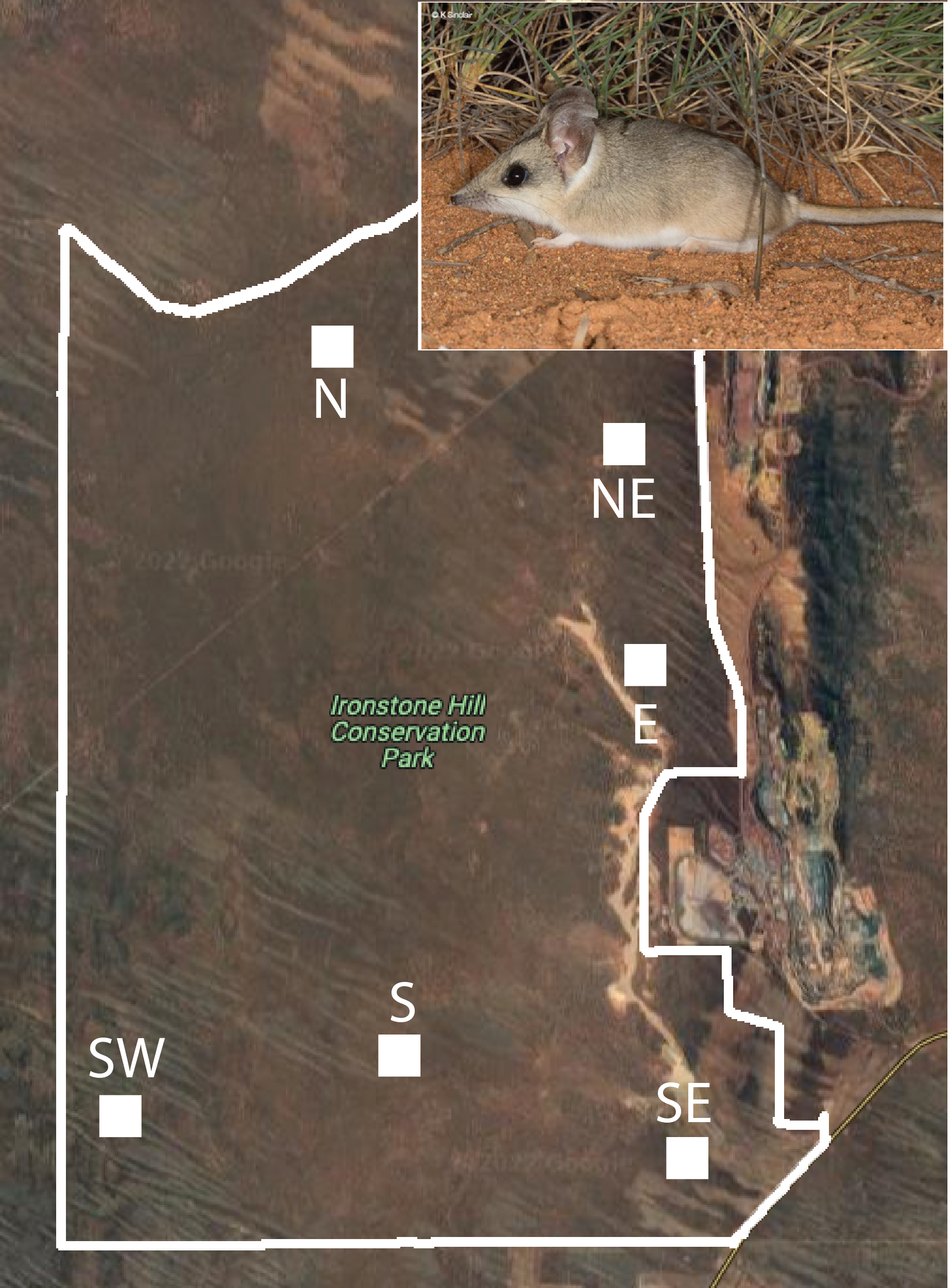
Researchers wanted to understand if the size of a vulnerable marsupial was related to local vegetation cover. This example measured body size (g) of mature female Sandhill Dunnards (Sminthopsis psammophila). Dunnarts were trapped and weighed in six subsections of the Ironhill Conservation Park west of Whyalla, South Australia, just before the onset of the September breeding season.
There are two continuous predictor variables:
- cover = Ground vegetation cover at the trap site (%)
- length = Dunnart length (mm)
The data are available in the file: dunnartData.csv. Save this into the "Data" folder of your CONS7008 R project before going any further.
dunnartData<-read.csv("Data/dunnartData.csv")
dunnartData$site<-as.factor(dunnartData$site) # make R treat site as a factor instead of a character
First, get an overview of the relationships between the predictor and response variables, and whether body mass is similar in different sampling sites:
## visually explore the data
pairs(dunnartData[,c("bodyMass", "cover", "length", "site")])
## what can we say just from looking at the pairs plot?

## are dunnarts similarly sized in the different areas?
with(dunnartData, boxplot(bodyMass ~ site))

## are sample sizes similar across sites?
table(dunnartData$site)
Were dunnarts at different sites similar?
No, dunnarts were smaller in east and south-east sites.
What 'level' were cover and length been measured at?
Length was measured for each individual dunnart, while cover was measured for each site (so that all dunnarts trapped in a given site have the same vegetation cover value).
Do we have similar sample sizes at each site?
No. There were fewer dunnarts trapped in east, north and north-east sites.
We might be tempted to just model using a linear regression.
## fit a linear model
dunnartCompPool<- lm(bodyMass ~ cover + length, data = dunnartData)

## let's look at some plot diagnostics using DHARMa
library(DHARMa)
plot(simulateResiduals(dunnartCompPool))

## if nothing looks too bad (which it doesn't), we can check the model summary
summary(dunnartCompPool)

## now hold on, let's go back and check those residuals again, this time looking
## for whether they're similar at each site
boxplot(residuals(dunnartCompPool) ~ dunnartData$site)
How does this model "pool" our observations?
This model is "complete pooling", where all observations are treated as one big group.
What would we conclude from this model?
Body length and cover are both positively associated with dunnart body mass. Also, This model explains ~47% of the variation in dunnart size in our data.
What are the issues with this model (hint: there are two)?
1. Dunnart size is related to site. We can't treat observations at the same site as if they're independent. This is clear in the model residuals, where residuals are strongly related to site.
2. We have different sample sizes at different sites. Sites with more dunnarts influence the model parameters more than those with fewer dunnarts.
Can we solve this problem by adding sites as a predictor in our model?
## fit a linear model
dunnartNoPool <- lm(bodyMass ~ cover + length + site, data = dunnartData)

## does this fix our issue with residuals being linked to site
boxplot(residuals(dunnartNoPool) ~ dunnartData$site)

## check the summary
summary(dunnartNoPool)
We've added a categorical predictor this model. What do the intercept and the "site" parameters mean?
The intercept is the mean body mass in the first level of the "site" factor (which is alphabetical unless we tell R otherwise, so "E" in this case). Each "site" parameter is the difference in mean body mass from the mean of the eastern site (intercept).
This model is appropriate if we want to estimate the size of dunnarts at each site. But if we want to get a more general population estimate across the whole conservation area, the above model can't give us this. This is because this model has "no pooling". Dunnarts from each site are separated and can't be used to make more general population estimates.
Given that dunnarts in our sites differ systematically across each site, but we don't want to explicitly estimate differences for each site, we could consider "partially" pooling site observations together in a mixed-effects model. In such models, site intercepts are treated as "random" intercepts. They are assigned their own normal distribution - that is, they are treated as being drawn from a "population" of possible site intercepts centred around some hypothetical "average" intercept. We can then examine the variance or standard deviation of this distribution, referred to as a "random effect". The fixed effects are the overall relationships that we are interested in. In this case they are the overall "average" intercept, and slope estimates for 'length' and 'cover'.
## install some new and exciting packages!!!
install.packages("lme4")
install.packages("performance")
install.packages("lmerTest")
install.packages("patchwork")

## load these (and DHARMa)
library(lme4) # for mixed-effects models
library(lmerTest) # to get p-values
library(performance) # a good package to measure model performance

## Mixed-effects model structure
dunnartPartPool <- lmer(bodyMass ~ cover + length + (1|site), data = dunnartData)

## diagnostics using the 'simulateResiduals' function in DHARMa
plot(simulateResiduals(dunnartPartPool))

## NOW! The mixed-effects model summary
summary(dunnartPartPool)

## we can get the "random" intercepts for each site like this
coef(dunnartPartPool)

## we can also estimate how much variance is explained by the fixed effects ("marginal R2") and fixed + random effects ("conditional R2")
r2(dunnartPartPool)
How can we tell what the random intercepts are doing?
The variance and standard deviation in the random effects of the model summary show us how variation in dunnart body is is structured. Site explains a lot of variation.
What are the random intercepts?
We see them in the "(Intercept)" column of coef(dunnartPartPool). Each site has its own intercept which is set alongside the slopes for cover and length to explain whatever LEFTOVER variation in bodymass is shared by dunnarts at the same site. Some sites have higher average biomass for reasons NOT EXPLAINED by vegetation cover and length, while others have lower average biomass.
You will notice the "cover" and "length" columns show the same coefficient estimates, and that these match the fixed-effect estimates in the model summary. These are the slopes, and they are the same because we only told the model to let the intercepts vary for each site, NOT the slopes. The online module has an example of what it looks like when you introduce "random slopes". If you ran a model like that, these slope estimates would also vary for each site just like the intercepts do.
How much variation in dunnart body size is explained by site?
**40.8% (conditional R2 - marginal R2)*100. Remember, the "conditional R2" is the variance explained by fixed + random effects, and the "marginal R2" is the variance explained by the fixed effects alone. So if we want to know how much variance the "random site intercepts" explain, its just conditional R2 - marginal R2.**
Now let's generate a plot. We're going to reuse the curve() function from previous pracs. We will also show you how to save these plots as pdfs using a function in R called pdf(). Note that using pdf() won't show you your plot in the plot window of RStudio, you will need to go to the location you save your file to see it!
pdf("Outputs/dunnartPopPreds.pdf", width=12) #this sets up a blank .pdf file in the ???Outputs??? folder called ???dunnartPopPreds.pdf???
# The plot you make will be ???projected??? onto this blank PDF

par(mfrow=c(1,2)) # we want two side-by-side figure panels

## plot the raw data as ugly open circles
with(dunnartData, plot(bodyMass ~ cover))

## add the regression slope
## (we need to use fixef() to get the "fixed effects"), coef() doesn't give us the overall intercept
curve(cbind(1,x,mean(dunnartData$length))%*%fixef(dunnartPartPool),
      from=min(dunnartData$cover), to=max(dunnartData$cover), add=TRUE,
      lwd=2, col="goldenrod")

with(dunnartData, plot(bodyMass ~ length))

curve(cbind(1,mean(dunnartData$cover),x)%*%fixef(dunnartPartPool),
      from=min(dunnartData$length), to=max(dunnartData$length), add=TRUE,
      lwd=2, col="goldenrod")

dev.off() # the PDF won't appear in your Outputs foler until you close the device, like this.
# NOTE if you re-run this code, it will overwrite the old version of your PDF! To make a new one you will need to change the file name


## We can make the same plots using ggeffects ('predict_response' function)
library(ggeffects)
library(tidyverse)
library(patchwork)## another nice package to arrange ggplots

## choose values of rainfall to plot the curves
cover_to_plot<-seq(min(dunnartData$cover), max(dunnartData$cover), length.out=200)
##  Now make the model predictions for the values we want
dunnart_cover_prediction<-predict_response(dunnartPartPool, terms = c("cover[cover_to_plot]"))


length_to_plot<-seq(min(dunnartData$length), max(dunnartData$length), length.out=200)
##  Now make the model predictions for the values we want
dunnart_length_prediction<-predict_response(dunnartPartPool, terms = c("length[length_to_plot]"))


dunnart_cover_plot<-plot(dunnart_cover_prediction, show_data = T, show_title = F)
dunnart_length_plot<-plot(dunnart_length_prediction, show_data = T, show_title = F)

## Now arrange and save them
dunnart_combined_plots<-dunnart_cover_plot + dunnart_length_plot

ggsave(file = "Outputs/dunnart_combined_plots.pdf",dunnart_combined_plots, width = 10, height = 5)
If we want to plot with our "random" site random intercepts, we can use site intercepts in coef(dunnartPartPool). This only makes sense for dunnart length, where we don't have a single value per site.
pdf("Outputs/dunnartSitePreds.pdf")

with(dunnartData, plot(bodyMass ~ length, col=site)) # colour points by site

## now we'll loop through our sites, generating a curve for each site
lapply(1:length(unique(dunnartData$site)),
       function(n){

      # we're looping through sites, let's get the data for just our site
      tempSite <- dunnartData[dunnartData$site == levels(dunnartData$site)[n],]

      # now here we're using the cover for the actual site, and we're using the
      # site-specific coefficients instead of the global coefficients from fixef().
      # This will give us site intercepts
      curve(cbind(1,mean(tempSite$cover), x) %*% unlist(coef(dunnartPartPool)$site[n,]),
            from=min(tempSite$length), to=max(tempSite$length), col=n, add=TRUE, lty= 2)

       })

## and let's add the overall average (fixed effect) intercept for good measure!
curve(cbind(1,mean(dunnartData$cover),x)%*%fixef(dunnartPartPool),
      from=min(dunnartData$length), to=max(dunnartData$length), add=TRUE,
      lwd=4, col="black")

dev.off()
This is not easy to implement in ggeffects, so we don't show you the equivalent approach here.
7.2 Nesting in experiments
Temperature induced bleaching of Acropora hyacinthus
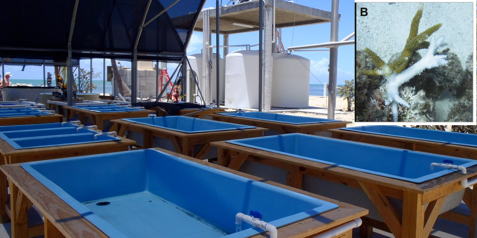
The effect of heat-induced bleaching on reef-building coral is well known and publicised. But bleaching is a response to multiple stressors, including temperature, disease, light exposure and nutrient deficiency. Understanding the physiological response of coral to warming water is challenging in the ocean, as local hydrology can alter water temperatures substantially from those sensed at the sea surface, and high temperatures often co-occur with high light conditions (sunny weather). Experimental studies of coral bleaching under controlled conditions provides an opportunity to study the bleaching sensitivity of important coral species.
This experiment, conducted at UQ's Heron Island Research Station, examined the effect of ocean warming on the bleaching of fragments of Acropora hyacinthus. Bleaching (cm\(^2\)) was measured for 120 fragments of A. hyacinthus suspended in small tubs, which were heated to one of three temperature treatments (26\(^\circ\), 28\(^\circ\) and 30\(^\circ\)C) for one week. This equates to 2000 AD summer mean water temperature as a control (28\(^\circ\)), with experimental treatments of -2\(^\circ\) (26\(^\circ\)C) and +2\(^\circ\) (30\(^\circ\)C).
Groups of 30 tubs (10 replicates of each temperature treatment) were grouped into raceways which circulate fresh seawater.
There is one categorical and one continuous predictor variable:
- tempTreatment = Temperature of seawater (\(^\circ\)C)
- fragmentSize = Surface area of A. hyacinthus fragment (cm\(^2\))
The data are available in the file: bleachingData.csv in the "Data" folder of our CONS7008 R project.
bleachingData<-read.csv("Data/bleachingData.csv", header = T, stringsAsFactors = TRUE) # this time we use "stringsAsFactors = TRUE" to tell R to treat character variables as factorsFirst, get an overview of the relationships between the predictor and response variables, and differences between experimental raceways.
## visually explore the data
pairs(bleachingData[,c("bleaching", "tempTreatment", "fragmentSize", "raceway")])
# what can we say just from looking at the pairs plot?

## Are bleaching levels similar across raceways?
with(bleachingData, boxplot(bleaching ~ raceway))

## Is the experimental design balanced?
table(bleachingData$raceway, bleachingData$tempTreatment)
Is bleaching related to raceway? If so, why might this be?
Yes. ON AVERAGE, there appears to be more bleaching in raceway B, and less bleaching in raceway C.
This could be caused by local environmental conditions at those raceways. They may be exposed to more light or naturally high temperatures from their location. Or, if the water in tubs is shared across the raceway, a diseased fragment may be infecting others. Or the raceway itself may have variation in water flow, or the sensors controlling water temperature may not be calibrated properly. There are so many reasons why experimental replicates might differ systematically, which is one reason why blocked designs are recommended.
What is the purpose of the 28\(^\circ\)C control?
Snapping off fragments of coral and suspending them in buckets is not really natural. The control is there to estimate the bleaching response to everything about the experiment that isn't water temperature. Thus we want to estimate changes in bleaching response from control rates.
As before, let's start with a simple regression.
## fit a linear model
bleachingCompPool<- lm(bleaching ~ tempTreatment, data = bleachingData)

## first - diagnostics.
plot(simulateResiduals(bleachingCompPool))
## Oh no, trouble!
Now we know that residual variation is still linked to raceway location, so let's update our model to a mixed-effects model.
## Mixed-effects model structure
bleachingPartPool <- lmer(bleaching ~ tempTreatment + (1|raceway), data = bleachingData)

## DHARMa diagnostics
plot(simulateResiduals(bleachingPartPool), asFactor=FALSE)
## looks like there's a problem! Some of our residuals deviate from expectations. What's going on?
How is this model treating the "tempTreatment" variable?
Currently tempTreatment in the bleachingData is a numeric variable (you can use str(bleachingData$tempTreatment) to see for yourself. Temperature is numeric, but we don't have a spectrum of temperatures, just three treatments. We want to have a categorical factor, with 28 as the reference level.
Is there anything else missing?
Well, we've measured bleaching in surface area units. Larger fragments have more area to bleach, so we might expect a correlation between fragment size and bleaching. This may interact with temperature treatment as well, so we should explore an interaction effect.
When fitting interactions between categorical and continuous predictor variables it often makes sense to centre the continuous predictor on its own mean (i.e. subtract the mean of the variable from each value). In this case, we subtract the mean fragmentSize from each value of fragmentSize so that the new mean is zero. This helps us understand the model output. Instead of the model estimates being calculated for fragmentSizes of zero (this doesn't make sense!), the model now calculates estimates for average fragmentSizes. That is far more sensible!
## convert temperature to a factor and choose the reference level we want
bleachingData$tempFact <- factor(bleachingData$tempTreatment,
                                 levels=c(28,26,30)) #28 goes first to be the "reference"

## use 'str' to check that R is treating it correctly
str(bleachingData$tempFact)

## centre the fragment size variable on its own mean
bleachingData$c_fragmentSize <- bleachingData$fragmentSize - mean(bleachingData$fragmentSize)

## look at a histogram of c_fragmentSize to see what happened
hist(bleachingData$c_fragmentSize)# the mean is zero!

## update model with treatment as a factor and fragment size
bleachingPartPoolCat <- lmer(bleaching ~ tempFact * c_fragmentSize + (1|raceway), data = bleachingData)

## diagnostics
plot(simulateResiduals(bleachingPartPoolCat)) # ahhh that's better.
Now we have a model with acceptable diagnostics! Just like a basic linear regression, there are multiple ways we can summarise the model results. First we will look at an ANOVA summary that conducts omnibus tests (i.e., it looks at overall effects of the variables and their interaction). You may have noticed earlier that we loaded the lmerTest package. This package includes a special version of 'anova' that works on mixed-effects models. By default, it uses a Type III ANOVA where each term (main effect or interaction) is tested after all other terms have been accounted for.
So we can see that the interaction is significant, and so is each main term. But this doesn't give us any of the model coefficients we need to try and interpret the results. We need to look at a "treatment contrasts" summary, like we did in previous weeks for simpler linear models. We can also "dig into" the model and grab the "random" intercepts for each raceway.
## treatment contrasts summary
summary(bleachingPartPoolCat)

## and the random intercepts
coef(bleachingPartPoolCat)

## and the model performance
r2(bleachingPartPoolCat)
Why is this model so much better than the earlier bleaching models?
The model that includes fragment size and its interaction with the treatment is far better at explaining variation in bleaching than the other two models. It also meets our statistical assumptions most strongly!
What does each line of the fixed effects summary show us?
(Intercept) = mean bleaching in our control group, at the average fragment size
tempFact26 = difference in mean bleaching from the control (28\(^\circ\)C) mean for the cooler temperature, at the average fragment size
tempFact30 = difference in mean bleaching from the control (28\(^\circ\)C) mean for the hotter temperature, at the average fragment size
fragSize = Correlation between fragment size and bleaching, in the control (28\(^\circ\)C) group
tempFact26:fragSize = Change in the slope of fragSize relationship in the 26\(^\circ\)C treatment
tempFact30:fragSize = Change in the slope of fragSize relationship in the 30\(^\circ\)C treatment
Is the raceway random effect necessary?
Yes, it explains LEFTOVER variation in bleaching, and the conditional R\(^2\) of the model is 10% higher than relying on the fixed effects alone.
Now let's generate a plot for our treatment levels. This is super easy these days with ggeffects.
## Make the predictions for each temperature
bleaching_prediction<-predict_response(bleachingPartPoolCat, terms = c("tempFact"))

## Plot them
bleaching_plot<-plot(bleaching_prediction, jitter = T, show_data = T, show_title = F)

ggsave(file = "Outputs/bleaching_plot.pdf",bleaching_plot, width = 5, height = 5)
7.3 Repeated measures study

Grassland productivity and the influence of climate change
Climate change is leading to irreparable damage to all scales of biological organisation, but especially to communities and ecosystems. But not every aspect is always negative, and in some cases, especially when organisms occupy marginal environments at the edge of their range limits, warming may actually improve growth rates.
To test the impact of warming on plant productivity, a field experiment was conducted in the Tasmanian alpine meadows of Granite Tor Conservation Area. Six plots of 2m\(^2\) (circle with 1.6m diameter) were established in each of six blocks. Three plots per block were enclosed with an open-top chamber which warmed the interior by approximately 3\(^\circ\)C. Dry-weight biomass in each plot was sampled by taking vegetation strips at four time intervals: at the start of the experiment (time 0), and at four-weekly intervals (1 = 4 weeks, 2 = 8 weeks, 3 = 12 weeks). The experiment started at the onset of the spring growing season, running for approximately three months.
There are two predictor variables:
- enclosure = inclusion of experimental warming chamber (categorical: Y or N)
- timeSample = which is effectively the number of months after the experiment started that each sample was taken
It make sense to include an interaction between these two predictors because we expect that the accumulation of biomass through time will vary DEPENDING ON the warming treatment.
The data are available in the file: biomassData.csv in the "Data" folder of our CONS7008 R project.
Let's explore our data.
head(biomassData)
## visually explore the data
pairs(biomassData[,c("biomass", "block", "timeSample", "enclosure")])
## what can we say just from looking at the pairs plot?

## Does biomass vary by block?
with(biomassData, boxplot(biomass ~ block))


## Plot biomass through time for each block using ggplot
biomass_time_plot<-ggplot(biomassData, aes(y = biomass, x = timeSample, col = enclosure, group = plot)) +
      geom_point() +
      geom_line() +
      labs(y = "Biomass (g per plot)", x = "Time (months)") +
      facet_wrap(~block, nrow = 2) +
      theme_bw()

ggsave(file = "Outputs/biomass_time_plot.pdf",biomass_time_plot, width = 10, height = 7)
How many random effects do we need in this model?
We need two.
Our experiment is clustered in space (in experimental blocks) and we expect plots within blocks to be more similar than plots from other blocks. This could be due to micro-environmental or nutrient levels, or even aspects of community composition.
As well as this, we have sampled within our plots multiple times so we need to account for this.
Let's run our model as a linear model to check.
## fit a linear model
biomassCompPool<- lm(biomass ~ enclosure * timeSample, data = biomassData)

# diagnostics (always)
plot(simulateResiduals(biomassCompPool))

# These are ok. We can examine the summary
summary(biomassCompPool)

# residuals by block
boxplot(residuals(biomassCompPool) ~ biomassData$block)

# residuals by sample time (our time predictor has explained most of the time variation)
boxplot(residuals(biomassCompPool) ~ biomassData$timeSample)
There is a lot of residual variation linked to block. Not good news for a model that assumes independence! So we know we need a mixed-effects model. We need to think about how to specify multiple random effects. In this case we need to NEST random effects within each other. If a normal mixed-effects model is like stacking our regular linear model on top of the group-level model (think back to the online module), then nesting two random effects is like stacking one group-level model on another (we have groups inside groups, like nesting dolls). In this case, we have multiple biomass strips (our "observations") taken within each plot, and our plots are clustered within blocks. We can specify this by altering the random effects in our model formula to look like + (1|block/plot), where the larger grouping variable comes first, then the smaller (nested) grouping variable. Equivalently, this can be specified as + (1|block) + (1|plot:block) where the ":" means "within" (so plot is nested within block in this case).
Let's give it a try!
# mixed-effect model with observations nested in plots, which are nested in blocks
biomassPartPool <- lmer(biomass ~ enclosure * timeSample + (1|block/plot), data = biomassData)

# DHARMa diagnostics
plot(simulateResiduals(biomassPartPool))

# model summary
summary(biomassPartPool)

# look at the random effects (look closely)
coef(biomassPartPool)
# there are two entries in this list ("$block" and "$plot:block") with different intercepts.

# mixed-effects models don't really calculate actual intercepts. They calculate "deviations from the global intercept", which we can see if we use ranef().

# global intercept
fixef(biomassPartPool)[1]

# and the intercept deviations from this global intercept (some are higher (positive) and some are lower (negative))
ranef(biomassPartPool)

# we can add the "intercept deviations" to the global intercept and compare them to coef()
cbind(coef(biomassPartPool)$block[,1],
      ranef(biomassPartPool)$block + fixef(biomassPartPool)[1])
# Hopefully it's clear that they're the same thing.
How do we explain the random effects section of the model summary?
As with the earlier mixed-effects models we fitted today, we have more than one error term. In this case we have 3! From the largest grouping variable to the smallest, these are: (1) Unexplained variance between blocks, (2) unexplained variance between plots (within blocks) and (3) unexplained variance within plots (residual). We can sum the variance like in the online module to determine what proportion of variation is being explained by each random effect.Which random effect explains most variation in biomass?
The residual (within plot) variance is the largest.So now we have a good model, let's plot the fixed effect relationships over the raw data.
## Make the predictions
grass_biomass_prediction<-predict_response(biomassPartPool, terms = c("timeSample", "enclosure"))

## Plot them
grass_biomass_plot<-plot(grass_biomass_prediction, jitter = T, show_data = T, show_title = F) +
  labs(y = "Biomass (g per plot)", x = "Time (months)") +
  theme_bw()

## save them
ggsave(file = "Outputs/grass_biomass_plot.pdf",grass_biomass_plot, width = 5, height = 4)
Look at the plot we just made, and the previous plot of biomass through time for each block (and plot therein). Might there be a problem assuming a linear relationship between time and biomass?
Focus on the patterns for the warming chambers especially. Notice how biomass values flatten off between time 2 and time 3 for quite a few plots? The linear fit does not capture this!7.4 Challenges:
Here you can extend some of previous scenarios to get you creating your own variables and models, using the functions from above. In each of these challenges, make sure to check model diagnostic plots and model summaries so you understand what the model is telling you.
Scenario 1: In this scenario we found that the body mass of dunnarts was related to their length. Create a new response variable that is mass divided by length (which is a mass to length ratio), and model this using vegetation cover as a predictor variable. Are your conclusions the same as the model we used above?
Scenario 2: We only tested up to 30\(^\circ\)C in this study, but we might want to predict bleaching at even warmer temperatures. Run a model with temperature treated as a continuous fixed effect, then predict bleaching surface areas at 31\(^\circ\) and 32\(^\circ\)C.
7.5 List of useful functions
Here are a few useful functions that you learned today.
Model predictions
emmeans::emmeans() Generate predictions and confidence intervals for categorical fixed effects
emmeans::confint() Extract the predictions and confidence intervals from an emmeans object
Statistical analysis
lme4::lmer() Fit linear mixed-effects models!
lme4::fixef() Get overall population intercept and slopes from a mixed-effects model
lme4::coef() Get the random intercepts of a model (as actual intercepts)
lme4::ranef() Get random intercepts of a model as deviations from the population intercept
DHARMa:simulateResiduals() Diagnostic plots for a great range of models including LMMs
Plotting
lapply() Like a loop but cleaner and nicer