Practical 3 Introduction to hypothesis testing
One of the most common class of questions that are asked in biology (including ecology and conservation science) is whether the mean of a sample differs from either a set value, or the mean of some other sample. For example, does giving patients a specific drug causes a change in the value of a response variable of interest (e.g., survival) compared to those who got the placebo?
We can easily calculate the difference of the mean of our sample from a fixed value (e.g., zero) or between two means (e.g., treatment and control groups). But, the mean of our sample is just an estimate of the true mean of the population, and we know that there will be some (hopefully small!) error in our estimate.
To determine whether or not our mean differs from another value or the mean of another group, we need to take that error into account. In this prac, we are focused on reinforcing your understanding of the principals of hypothesis testing in science. We will use a specific analysis, the t-test, to really dissect the basis of testing biological hypotheses using any form of statistical test.
In this practical you will:
- explore the idea of a "test statistic" through a detailed study of the t-test;
- use the t-test to clarify the concepts of "null hypothesis" and "alternative hypothesis";
- use the t-test to clarify the concepts of "statistical power", "Type I error" and "Type II error", and;
- you will apply your knowledge to this question: "How can one judge the relative merits of separate studies that address the same question"? You will be able to finally decide whether to recommend that Team A or Team B receive the additional $15M in funding to develop their cancer treatment drug, Cureallaria!
3.1 Hypothesis testing

A tea party
In an afternoon tea break with Ronald Fisher, phycologist Muriel Bristol claimed to be able to tell whether the tea or the milk was added first to a cup.
Fisher hypothesised that Bristol couldn't tell the difference, and he wanted to test his hypothesis.
If Fisher handed Bristol a cup of tea and asked her: "did the tea or milk go in first?" then Bristol would have a 50% chance of guessing correctly. If Fisher made two cups, there would still be a high chance that Bristol could guess correctly twice.
Fisher decided to test Bristol with eight cups, four of each variety, in a random order. One could then ask: what is the probability of Bristol correctly guessing the four that had her preferred milk-first tea? Fisher calculated this probability as 1 in 70 (4/8 * 3/7 * 2/6 * 1/5 = 24/1680 = 1/70 = 1.43%). While it is possible to guess all eight correctly, it is unlikely.
Needless to say, Bristol got all eight correct!
Fisher was convinced, and concluded that Bristol could tell the difference - he rejected his original ("null") hypothesis.
NB: This story summarises the hypothesis testing framework; the "tea" from the party is different to the "t" from the t-test. Fisher went on to become one of the most influential bio-statisticians of all time, among other things, establishing the fundamentals of experimental design and ANOVA. We'll never know what you would be studying right now if Muriel Bristol hadn't been so (rightly!) confident in her ability to taste scalded milk!.
3.1.1 Null and alternative hypotheses
Statistical hypothesis testing in biology (and other fields!) depends on two cornerstones. First, that we can state a null hypothesis. Typically, we frame the null hypothesis as there being "no difference" (e.g., the means of two treatments are the same). When we reject our null hypothesis, we interpret this as support in favour of an alternative hypothesis.
The alternative hypothesis is mutually exclusive with the null, stating that a population parameter is not the same as some hypothesised value (e.g., the means of two treatments differ). The alternative hypothesis could be that the population parameter is greater or smaller (one-sided) than the hypothesised value, or that the population parameter is different (either bigger or smaller: two-sided) to the hypothesised value.
What were the null and alternative hypotheses in Fisher's test?
Null hypothesis: Bristol cannot tell the difference.
Alternative hypothesis: Bristol can tell the difference.
Fisher rejected the null hypothesis that Bristol could not tell the difference.
Is the alternative hypothesis definitely true?
Never!
It is still possible, albeit unlikely, that Bristol guessed correctly 8 times. While a well-designed experiment can allow us to draw conclusions about the probability of observing the data we have if the null hypothesis was true, we cannot prove that the alternative is true.
We can think about statistical hypothesis testing as Fisher laid out - what is the probability of observing our sample data (8/8 correct guesses) if the null hypothesis is true? Here, if Bristol could not taste the difference between teas (i.e., the null hypothesis is true), the probability of correctly identifying all 8 cups is 1.43%
Recalling the cure for cancer studies that you analysed in Practical 2, what null hypothesis do you think that Team A had?
What null hypothesis has the Minister tasked you with addressing?
Within each study (Team A or Team B), researchers are testing the null hypothesis that mean survival is the same for the Control and Cureallaria treatments, that is, the treatment has no effect on survival.
The Minister is asking you consider which research team should be further funded. Your null hypothesis then is that the difference in mean survival between the Control and Cureallaria groups for Team A is the same as the difference in mean survival between the Control and Cureallaria groups for Team B. Only if we reject that null hypothesis do we have any basis for then asking "Why?" and delving into which team's preliminary results we trust to provide a better estimate of the average effect of the drug on survival.
3.2 Using test statistics
Once you have a hypothesis, a critical ingredient to test it is a test statistic. A test-statistic will follow some probability distribution (e.g., Gaussian, t-distribution, exponential). That is, test statistics have a special property: We know what kinds of values to expect of them when the null hypothesis is true. Because we know the probability distribution for a test-statistic, they also have the converse property: We know what values they won't have when the null hypothesis is false!
This is all a bit abstract but you have encountered test statistics before, including the t-statistic (used in a t-test) and F-statistic (used in ANOVA).
Here is the calculation for the t-statistic for a one-sample test:
\(t = \frac{m - \mu}{s /\sqrt n}\)
\(m\) is the sample mean;
\(\mu\) is the "population" mean (a hypothetical value that you're testing against);
\(s\) is the standard deviation;
\(n\) is the sample size.
What value to you think that t is expected to take when the null hypothesis is true?
Zero! The statistic is calculated by subtracting the value we are testing against from our population parameter estimate (i.e., the value of the thing we care about). The null hypothesis is typically "no difference"; here, if our null hypothesis was true, and the values were the same, the difference is equal to zero.
When the null hypothesis is exactly met, then the denominator of this equation does not matter - zero over anything will equal zero. However, our estimate of the test statistic is unlikely to ever be exactly zero, even when the null hypothesis is true.
If your sample mean is larger than the population mean you are comparing to, would your t-statistic be positive or negative?
Positive! You are subtracting the hypothetical population mean from your observed sample mean.
What is the relationship between sample size and the t-statistic?
Remember, we need to consider uncertainty due to small sample size in addition to just looking at the difference between mean values. Smaller sample size increases the denominator of the t-statistic (the standard error) and thus decreases the t-statistic. Therefore, smaller sample size indicates that the observed difference in mean values may not be so meaningful.
3.3 Estimating the test statistic
Let's estimate the t-statistic for the cancer drug trials. First, we need to read in the data:
## read in the data and call it "cancer_data"
cancer_data<-read.csv("Data/Cureallaria.csv", stringsAsFactors = TRUE) ## using "stringsAsFactors = TRUE" forces R to convert character variables to factors (it is useful most of the time)
Remember, Team A included ten Controls and ten Cureallaria treatments, while Team B only included 3 of each. To demonstrate the various calculations involved in a t-test, we will do the calculations one step at a time, but please be assured that there are much faster ways of doing this. We will show you these later. First, let's use some functions from the Tidyverse to quickly do the required calculations for each combination of Team and Treatment. The Tidyverse uses slightly different syntax to base R, but it is very logical once you get used to it (probably more logical than base R!!!). The bits that look strange at first glance are the %>%. These are called "pipes" and they just mean "then do this next thing...".
library(tidyverse) ## load the Tidyverse package

## We will plot 95% confidence intervals around our treatment means
n.se <- 2 ## This is the number of standard errors (either side of zero) that typically captures 95% of the t-distribution

## we will create a summary dataframe called "cancer_summary_data"
cancer_summary_data<-cancer_data %>% ## start with cancer_data, then do this next thing...
  group_by(Team, Treatment) %>% ## group the data based on Team and Treatment, then do this next thing...
  summarise(cured_means = mean(N_cured_from_100), ## now for each combination of Team and Treatment, do some calculations
            cured_SDs = sd(N_cured_from_100),
            group_Ns = length(N_cured_from_100))%>%
    mutate(cured_SEs = cured_SDs/sqrt(group_Ns), ## now use "mutate" to make a couple more variables including standard errors
           cured_95_CIs = cured_SEs * n.se ## also multiply the SEs by 2 for plotting 95% CIs
  )

## now look at what you just made!
cancer_summary_data
Which team (A or B) observed the biggest average effect of the treatment? We simply have to subtract the mean for Cureallaria from the Control mean for each Team.
For A: 65.5 - 39.9 = 25.6, whereas for B: 76.7 - 36.3 = 40.4
The value of the test statistic (t) depends not only on this difference in mean, but also on the standard error (the denominator in the equation: standard deviation divided by the square root of the sample size).
The standard error (SE) tells us how confident we are in the estimate of the parameter. In this case, if our Cureallaria mean is different to the Control mean, but the variation in values is large (high SE), then we are unlikely to conclude that the Cureallaria treatment is actually different to the Control (we can't reject the null hypothesis).
To think about this further, let's plot the cancer study data using means and SEs to visualise what is happening when we do a t-test. Plotting this in base R is VERY cumbersome. Here we will use the ggplot function from the Tidyverse. Again, the syntax for ggplot is slightly different to plotting in base R, but we can get beautiful plots MUCH quicker using ggplot. In ggplot, we start by telling it what data we want to use (the "cancer_summary_data" we just made), and then we tell it some "aesthetics", including which variable we want on the x-axis, which one we want on the y-axis, and which variable we want to treat as an additional group. Then we tell ggplot what kinds of things we want to plot. These are referred to as geometries, or "geoms". In this case we want to plot points for means and lines for error bars, so we use geom_pointrange. Notice how we use + to keep adding things to a ggplot. We will explain what else is happening once we have all made the plot.
ggplot(data = cancer_summary_data, aes(x = Team, y = cured_means, group = Treatment, colour = Treatment)) +
  geom_pointrange(aes(ymin = cured_means-cured_95_CIs, ymax = cured_means+cured_95_CIs),
                  position = position_dodge(width = 0.25)) +
  ylab("Number cured (from trials of 100 people each)")
Looking at the confidence we have in the mean of the Control versus Cureallaria, do you think that a t-test might reject or accept the null hypothesis? Does your conclusion depend on which team you are considering?
The means of the two Treatments for each team do seem distinct, so it seems that a t-test might reject the null hypothesis. However, the confidence intervals for Team B's estimates are quite a lot wider, so it might be more difficult for Team B to detect the difference, despite their difference actually being a bit larger!
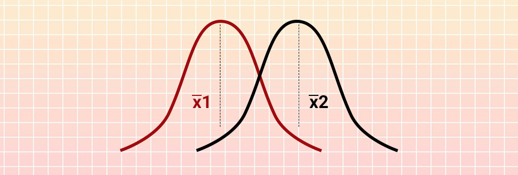
Because t is is calculated by dividing a difference in means by a standard error, we can think of t values as differences divided by our uncertainty in their estimation. If differences are large and we are very certain of their values, then we are dividing a large difference by a small standard error, which creates large t values.
As you can see in the figure below, the t distribution is centred on zero because it is a representation of the null hypothesis (that there is no difference). If our observed t is well away from zero, then we are confident that the difference is not zero and we can reject the null hypothesis.
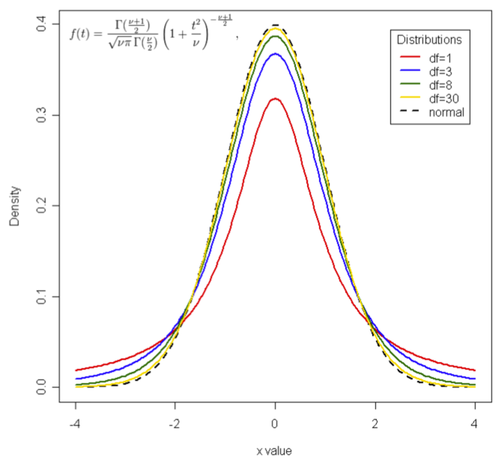
Even though the t distribution changes depending on the degrees of freedom (as shown above), the bulk of the t distribution does not change that much with the degrees of freedom. Indeed, when the null hypothesis is true most values of t fall between -2 and +2. Therefore, as a "rule of thumb", when our t value is between -2 and +2, we probably cannot reject the null hypothesis. In other words, our t statistic will likely fall within the "do not reject" zone of the t distribution.
Let's go ahead and check our "guess" about whether we can reject our null hypothesis of no effect for this cancer drug study.
3.4 One sample t-test
One way to test the null hypothesis (Cureallaria = Control) would be to treat the mean of the Control group as a fixed reference value, and test whether the Cureallaria mean equals that fixed reference value. This approach is known as a "one-sample" t-test because we have only one sample of interest.
Team_A_subset_summary_data<-subset(cancer_summary_data, Team == "A") ## First, make a subset so that we are just looking at Team A summary data
Team_A_Effect_Size <- diff(Team_A_subset_summary_data$cured_means) ## calculate the difference in treatment means for Team A
Team_A_Cureallaria_SE <- Team_A_subset_summary_data$cured_SEs[2] ## grab the SE for the Cureallaria treatment (for Team A)
Team_A_One_Sample_t_stat <- Team_A_Effect_Size / Team_A_Cureallaria_SE  ## now calculate the t-stat

Team_A_One_Sample_t_stat  ## Look at the value of the t-statistic
OK! Based on our rule-of-thumb, do we think that this is going to fall within the bulk of the t-distribution, or in the 5% tails? Is this t-value consistent with what you expected from the plot?
To determine the probability of observing a t-value at least as extreme as the one that we have observed, we need to compare our observed value to the t-distribution for our degrees of freedom. R can do that for us.
## first, grab the mean for the Control treatment for Team A (as the fixed "reference" value)
Team_A_Control_mean <- Team_A_subset_summary_data$cured_means[1] ## It is the first mean in the summary data subset

## Now, make a subset of the "full" cancer data that only has the Cureallaria treatment for Team A
Team_A_Cureallaria_subset <- subset(cancer_data, Team == "A" & Treatment == "Cureallaria")
## The t-test function in R uses the original data values, not our pre-calculated effect size and SE

t.test(Team_A_Cureallaria_subset$N_cured_from_100, mu = Team_A_Control_mean)  ## Use R's inbuilt function to implement this one-sample t-test.
## Here, "mu" is a fixed value against which we test whether the observed Cureallaria values differ.
Should we reject our null hypothesis?
Yes!
Our t-statistic is larger than we would expect to see if our null hypothesis was true. Indeed, the probability of observing a t-value of 4.459783 or larger is 0.0016 (i.e. only 0.16%!).
3.5 Two sample t-test
The previous analysis has an obvious problem: the mean of the Control group is not really a fixed constant. Rather, it is itself an estimate subject to sampling error. A more appropriate analysis would consider the difference between the sample means of the two groups as the test statistic subject to sampling error. That is, we need to estimate the SE of that difference, not just the SE of the Cureallaria mean. Fortunately, there is an easy formula for calculating a standard error for that statistic:
\(SE=\sqrt{SE_1^2 + SE_2^2}\)
Team_A_Joint_SE <- sqrt(sum(Team_A_subset_summary_data$cured_SEs^2))  ## Standard error of the difference between the two means
Team_A_Two_Sample_t_stat <- Team_A_Effect_Size / Team_A_Joint_SE  ## now calculate the t-stat

Team_A_Two_Sample_t_stat ## look at the resulting value

## Now do the two-sample t-test using R's function
## first, make a subset of the "full" data that is just Team A (but including both the Control and Cureallaria treatments)
Team_A_subset <- subset(cancer_data, Team == "A")

## Now run the t-test in R - here we use the "formula" syntax: N_cured_from_100 ~ Treatment
## This just means we are asking R the question "does N_cured_from_100 differ by Treatment"
t.test(N_cured_from_100 ~ Treatment, data = Team_A_subset)
Now that you are appropriately accounting for the uncertainty in both sample estimates (Control and Cureallaria), do you accept or reject the null hypothesis?
Reject!
So we know that Team B had a larger effect size than Team A (40.3 versus 25.6), but had a much smaller sample size (3 versus 10). How did this affect conclusions when Team B's data were analysed properly using a two-sample t-test?
Team_B_subset<-subset(cancer_data, Team == "B") ## subset the cancer data to just look at Team B

t.test(N_cured_from_100 ~ Treatment, data = Team_B_subset) ## Now the t-test
Interesting! Team B was not able to reject the null hypothesis! Below we will dig deeper into the reasons why.
Assumptions of the t-test
As with ALL statistical analysis, we make some assumptions when interpreting the results of a t-test. If our data violate these assumptions, our conclusions might be wrong (more on that below). We will not consider these assumptions further here; in future practicals in the course, you will learn how to check for violation of model assumptions.
- The "residuals" (the "unexplained" part of the data, i.e., the "background noise") are Gaussian ("normally distributed"). In future practicals you will learn how to test this assumption, which is common to most "parametric" test statistics. When the data are very non-normal in distribution (e.g., skewed, or containing extreme outlier values, or multi-modal), the results of the t-test can be unreliable. However, the t-test is quite robust to violations of this assumption.
- The variance of the residuals is equal everywhere in the data. That is, we assume that different groups have the same variance. Again, although very large differences in variance can make our test unreliable, t-tests can be quite robust to moderate differences in variance. Notably, the chance of making an error in your conclusions from a t-test is greater if the sample sizes of your groups are uneven. Therefore, it's always important to try to design your data collection to attain similar sample sizes for groups that you want to compare.
- The separate measurements are made on independent random samples of the population. This assumption must be considered at the experimental design stage, before data are collected. Violations of this assumption impact on the generality of our conclusions. If our sample is not random, then repeating the analysis with a different sample might give a different result, and our conclusions might not be general to the population. In this context "independent" means that the individual samples are not related to one another in some way (e.g., multiple measurements taken on the same person will be similar to one another). We will discuss independence more later in the course, and show you tools to deal with correlated samples.
3.6 Type I and type II errors
Imagine it's the dying seconds of the AFL grand final. Your team, the Hawthorn Hawks, lead by two points. The ball is in their defensive goal square. One of the opposition players is possibly fouled by being pushed in the back. The umpire can do one of two things: pay a free kick, or not pay a free kick.
There are four outcomes:
the opposition player was pushed in the back AND the umpire pays a free kick (boo, but good work umpy, correct decision);
the opposition player was not pushed in the back AND the umpire pays a free kick (boo, get your eyes checked umpy!);
the opposition player was pushed in the back AND the umpire does not pay a free kick (YES!! You're a legend umpy - you'll help the Hawks win even though you were wrong);
the opposition player was not pushed in the back AND the umpire does not pay a free kick (YES! Good work umpy).
The point is this: we can't make one decision and it be right all of the time!
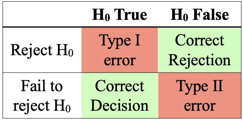
When we, as applied statisticians, accept or reject a null hypothesis, we are making a judgement. As professionals, we should generally make the right decision (just like the umpire - too many wrong decisions and they'd be out of a job!). However, sometimes, we might fail to reject the null hypothesis when it is false (false negative; type II error), or reject the null hypothesis when it is true (false positive; type I error).
Experimental design, and approaches to data analysis aim to find the appropriate balance between the risk of type I versus type II errors. Since scientists are often 'trying' to show an effect, type I errors are typically considered to be the more serious offense - but this isn't always the case. Here is a particularly horrendous example of a Type II error:
Rofecoxib (Vioxx, Merck)
Rofecoxib was a non-steroidal anti-inflammatory drug developed by Merck. It was a booming drug in the late '90s, but there was some suggestion that it may cause heart attacks.
By December 2000, 21 placebo-controlled trials had been performed. They suggested that Rofecoxib was 2.18 times more likely than placebos to cause serious heart problems or death. However, confidence intervals for this relative risk measure ranged from 0.93 (i.e., slightly less than the placebo) to 5.81 (almost six times more likely). The probability that the relative risk was significantly greater than one was P = 0.07. Hence, Merck accepted the null hypothesis of no difference between treatment and control groups.
Larger experiments that followed indeed found Rofecoxib to be almost twice as deadly as placebos. By the time it was taken off the market in September 2004, 20 million Americans had taken the drug; 88,000 had serious heart attacks; 38,000 had died.
Ross et al 2009
If Bristol couldn't tell the difference between tea first or milk first, which type of error did Fisher make?
Type I error. He rejected the null hypothesis, even though it was true.
In relation to hypothesis testing, errors are, simply, when the wrong decision is made. The probability of making the wrong decision is referred to as an "error rate". What affects error rates? Statistical power!
3.7 Statistical power
Statistical power has a very technical definition (explained in the pre-recorded statistics module) that typically confuses students. It can simply be thought of as our ability to detect a difference between groups IF A DIFFERENCE ACTUALLY EXISTS. A power value of at least 0.8 (or 80%) is considered desirable. The probability of committing a type II error is 1 - power, so if power = 0.8, then we have only a 20% chance (0.2 probability) of committing a type II error (failing to detect a difference that actually exists, or in more technical and confusing terms, failing to reject the null hypothesis when it is false).
Let's go through a simple example about forests (the best kind of example!) to understand power better. Imagine that there are two forests, each with 2 million trees, and the mean tree height of the first forest is 1 m taller than the second forest (i.e., if we were able to measure the height of ALL trees in both forests we would find this small difference). But, typically we don't have the time or money to measure every tree, so we take samples. For example, we might measure the heights of 500 randomly selected trees in each forest. Or we might be really lazy and only measure 10. Based on the samples we take, we might detect the difference or we might not, depending on the nature of our samples and the size of the difference we are trying to detect (small differences are harder to detect than large ones).
Statistical power has three "ingredients":
Effect size (the ACTUAL difference in average tree heights between the two forests that we are trying to detect with our samples);
Sample standard deviation (the variability of tree height values measured (sampled) in each forest); and
Sample size (the number of trees measured (sampled) in each forest).
We can explore this example using a simple ShinyApp. ShinyApps are built using R! But, we don't need to write the code and run it. Many people have built ShinyApps, and they are particularly useful for exploring parameter spaces to learn statistics.
Open the link below in a new browser:
http://shiny.math.uzh.ch/git/reinhard.furrer/SampleSizeR/
Click on "Power calculations: t tests". Use the default settings of "Unpaired", "Equal variance" and an alpha (\(\alpha\)) value of 0.05.
Now, the ACTUAL difference in average tree height (the effect size we are trying to detect) is 1 m. Let's say that the standard deviation of the measured trees in our sample is 2.5 (and we assume this is the same for both forests).
How many trees do we need to measure in each forest to achieve our desired power of 0.8?
100 trees per forest.
Now imagine that the tree heights in our samples were more variable and the standard deviation was more like 3.5. What power would we achieve now if we take 100 samples per forest?
Just over 50%. We would need to measure almost 200 trees per forest to achieve adequate power if the standard deviation was 3.5.
3.8 The power of the t-test
The generic R function power.t.test calculates the power of a t-test for a difference between two means. Let's apply it to Team A's cancer study data.
power.t.test(                                ## Calculate Power of T-test, and output the variable set "NULL"
  n = Team_A_subset_summary_data$group_Ns[1],   ## Sample size of each group
  delta = Team_A_Effect_Size,                 ## Difference between the means (effect size)
  sd = mean(Team_A_subset_summary_data$cured_SDs), ## Set a common standard deviation (using the average makes sense)
  sig.level = 0.05,                           ## Set a significance level (Type I error rate)
  power = NULL,                               ## Leave the power argument as NULL so that R calculate this for us
  type = "two.sample",                        ## Request a T-test comparing means of two groups
  alternative = "two.sided"                   ## Alternative hypothesis: Cureallaria survival is different to the Control
)
What does "power = 0.8530232" mean?
Given an effect size of 25.6, Team A's SD and a sample size of 10 per group, the probability of correctly rejecting the null hypothesis is 0.8530232.
Calculate the required information for Team B and input this into the power.t.test function.
Which team has the lower power (higher probability of committing a type II error)?
Team B!
The following R code produces graphs that relate effect size and sample size to power for the cancer data. The first relates effect size to power, for a given sample size. Lets see how big the effect size needs to be in order to get an acceptably high power.
EffectSize <- seq(0, 40, 1)           ## Set various effects sizes
Power <- NA                           ## Empty vector to hold the power estimates

for(i in 1:length(EffectSize)){       ## Loop through the effect sizes
Power[i] <- power.t.test(             ## Record the output at the "ith" place in "Power"
n = 10,                               ## Set the sample size of each group
delta = EffectSize[i],                ## Difference between the means (effect size)
sd = mean(Team_A_subset_summary_data$cured_SDs),                   ## Set a common standard deviation
sig.level = 0.05,                     ## Set a Type I error rate
power = NULL,                         ## Set the statistical power (1 - Type II error rate)
type = "two.sample",                  ## Request a T-test comparing means of two groups
alternative = "two.sided")$power      ## Alternative hypothesis: Cureallaria survival is different to the Control
}                                     ## Output the element called "power", then re-loop


plot(EffectSize, Power)   ## Graph power against effect size
abline(h=0.8, col="red") ## a red line indicate power of 0.8
What does an effect size of 10 mean?
The difference in survival between Control and Cureallaria treatments is 10. The drug improves survival by 10%.
How much power does Team A have to detect an effect size of 10?
Given their sample size (n = 10), about a 20% chance. In other words, the probability that Team A would fail to find this effect (type II error) would be 80%.
Now produce a second graph relating sample size to power. We set the effect size to the one "Team A" actually obtained.
SampleSize <- seq(2, 30, 1)                 ## Set various sample sizes
Power <- NA                                 ## Empty vector to hold the power estimates

for(i in 1:length(SampleSize) ){            ## Loop through the sample sizes
  Power[i] <- power.t.test(                   ## Record the output at the "ith" place in "Power"
    n = SampleSize[i],                          ## Set the sample size of each group
    delta = Team_A_Effect_Size,  ## Difference between the two means
    sd = mean(Team_A_subset_summary_data$cured_SDs),                         ## Set a common standard deviation
    sig.level = 0.05,                           ## Set a Type I error rate
    power = NULL,                               ## Set the statistical power (1 - Type II error rate)
    type = "two.sample",                        ## Request a T-test comparing means of two groups
    alternative = "two.sided")$power            ## Alternative hypothesis: Cureallaria survival is different to the Control
}

## Output the element called "power", then re-loop
plot(SampleSize, Power)         ## Graph power against sample size
abline(h=0.8, col="red") ## a red line indicate power of 0.8
What sample size per group should leave Team A confident of not making a Type II error?
If we aim for power of 0.8, then a sample size of about 7 or more would suffice.
In practice, we can really only increase power by increasing sample size (to improve the precision with which we have estimated the sample mean) - we cannot control how large the effect of the drug is (indeed determining how much it affected survival was the purpose of the study!!). We often use pilot studies or results from similar studies to estimate the likely effect size and sample standard deviation, from which we can estimate a sample size that should deliver sufficient power. In other situations, policies might dictate the effect size that needs to be detected in order to trigger some action. For example, policy might dictate that a 15% reduction in fish biomass on a given reef triggers the closure of that area to fishing. In this case, the smallest effect size that we need to try and detect is 15%. So understanding power is extremely important, not just for statisticians, but also for professionals gathering information to guide management.