Practical 5 Linear models - Analysis of Variance (ANOVA)

In this practical we are focused on another "flavour" of linear model - one that you will know as an Analysis of Variance (ANOVA).

ANOVA is the name given to linear models that include a continuous response variable and one or more categorical predictor variables(s). Remember, categorical variables define categories or groups, e.g. "Ambient" versus "Warmed" or "Not bleached" versus "Bleached". In statistical models, R treats these as "factor" variables with the different categories referred to as "levels". One-way ANOVA involves just one categorical predictor variable, though the predictor can have more than two levels. For example, an ANOVA involving a predictor with three levels (e.g. "Ambient", "Dry" and "Wet") is still just a one-way ANOVA. Two-way ANOVA involves two categorical predictor variables (each with two or more levels), three-way ANOVA involves three categorical predictor variables, and so on. There are two general types of categorical predictors that ANOVA can be applied to:

"nominal", with no intrinsic ordering to the categories (e.g., "Male" versus "Female"), or;
"ordinal", with a natural order to the categories (e.g., "Short" versus "Medium" versus "Tall").

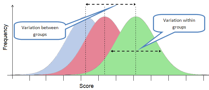
Irrespective of the number of levels in the predictor, the overall question that an ANOVA asks is "Do the different levels of the predictor variable account for significant variation in the response variable?" To answer this question, a single F-test is applied to test the null hypothesis that the mean of the response variable is the same across all levels of the predictor variable (i.e. all groups have the same mean response value).

If we reject that null hypothesis, we accept the alternative hypothesis that the mean of at least one level differs from the others. We can then proceed with subsequent tests to see which levels differ from each other in their mean response values.

In this practical you will:

Apply and interpret the results of "one-way ANOVA" linear models with one categorical predictor variable; and
Apply and interpret the results of "two-way ANOVA" linear models with two categorical predictor variables.

Assumptions of Linear Models with Categorical Predictors and Continuous Response Variables

The same general assumptions of linear models apply to ANOVA. Remember that they are:

The residuals have a normal (Gaussian) distribution;
The residual variance (variance within groups) is constant. In other words, the variance within each group is (approximately) equal. This assumption is violated if the spread of response values in one group is much wider than in other groups. It is the same assumption as in linear regression (that residual variance is constant across all values of \(X\));
Each measurement of the response variable is taken independently of every other measurement of the response variable.

5.1 Simple example of ANOVA

Open your CONS7008 R Project and set up a new blank script for today's prac.

We begin by analysing a very simple data set again, to orient you to how the analysis works, and to demystify the meaning of the numbers that R sends to the screen.

## Enter these made up numbers:
water_loss <- c(1, 2, 3, 4, 3, 4, 5, 6, 5, 6, 7, 8)

## Enter their treatment groups:
wind_speed <- rep(c("Low", "Med", "High"), each = 4)

## cbind together as a data frame
Simple <- cbind.data.frame(water_loss, wind_speed)  
Simple  ## View the data
summary(Simple)## how is R treating each variable?

What does rep(c("Low", "Med", "High"), each = 4) do?

It creates a new vector with the treatment groups, "Low", "Med", and "High", with each repeated 4 times.

Plot the data to see what we are working with. Here we do this very manually and incrementally. In the future we will show you easier plotting code but it's important to learn the basics first.

## Create x-axis locations for the "wind speed" levels
x <- rep(1:3, each = 4)

## Draw a scatter plot of "water_loss" versus "x" without axes
plot(x, Simple$water_loss, xaxt = "n", ylab = "Water loss", xlab = "Wind speed", cex = 1.5)

## Now add a customised axis
axis(side = 1, at = 1:3, labels = c("Low", "Medium", "High"), cex = 2, cex.axis = 1.75)

Which aspect(s) of the graph tells you that 'wind_speed' predicts 'water_loss'?

The dots tend to rise as you scan from left to right, with water loss low when wind speed is low and high when wind speed is high.

Which aspect(s) of the graph tells you that 'wind_speed' is not the only thing that affects 'water_loss'?

Within each level of 'wind_speed', there is a range (spread) of values of 'water_loss'.

Before we statistically analyse the data, we need to tell R how to treat our "wind_speed" variable. If we leave it to R, it will order the levels of wind_speed alphabetically as "High", "Low" and "Med" which is not ideal! We can force R to think like us instead!

Simple$wind_speed<-factor(Simple$wind_speed, levels = c("Low", "Med", "High"))

summary(Simple)## Did R obey our command?

Now we can analyse the data in a way that makes a bit more sense (stats can be confusing enough).

fit_simple <- lm(water_loss ~ wind_speed, data=Simple)   ## Fit a linear model
anova(fit_simple)                           ## Generate an ANOVA table

NB: R agrees with us that ANOVA is just one type of linear model - notice how the function that fits our ANOVA model, lm is the SAME function that we used to fit the linear regression model!!!

Which aspect of the ANOVA table tells you that 'wind_speed' affects 'water_loss' significantly?

The large F-statistic (and small P-value) for 'wind_speed'.

Which aspect of the ANOVA table tells you that 'wind_speed' is not the only thing that affects 'water_loss'?

The residual variance (Residual Mean Sq) is not zero.

5.2 The SAME model summarised using "model coefficients" instead of an "ANOVA table"

Our model (fit_simple) is just a linear model. We can summarise it's output in a couple of different ways. Above we looked at an ANOVA table that presents the "overall" test of whether one group's mean is different to any of the others (it doesn't tell us which group differs, or how it differs!!!).

To dig a bit deeper, we can look at a summary of the "model coefficients", just like we did for our linear regression last week. But first we need to understand how R treats categorical variables "under the hood" in the linear model. For each level, R creates a separate "dummy variable" that codes the observations as zeroes and ones. In the case of our wind_speed variable, R creates three dummy variables, one each for "Low", "Med" and "High". R will use the first category as a baseline or reference to which the other categories are compared. We have already told R our preferred order, so "Low" is first, and is defined as the "Intercept", then "Med" and finally "High". We can see EXACTLY how R is treating our wind_speed categorical variable by looking at the model matrix of fit_simple:

model.matrix(fit_simple)## see how R is actually treating the different categories in the fit_simple model

Now we understand what R is doing, we can look at the summary of model coefficients:

summary(fit_simple)## look at summary of model coefficients and associated t-tests

How should we interpret the estimate of 2.5 for "(Intercept)"?

The "Intercept" represents the average water loss for "Low" wind speed.

How should we interpret the estimate of 2 for "wind_speedMed"?

This is the difference in average water loss for "Med" wind speed relative to "Low" wind speed.

How should we interpret the estimate of 4 for "wind_speedHigh"?

This is the difference in average water loss for "High" wind speed relative to "Low" wind speed.

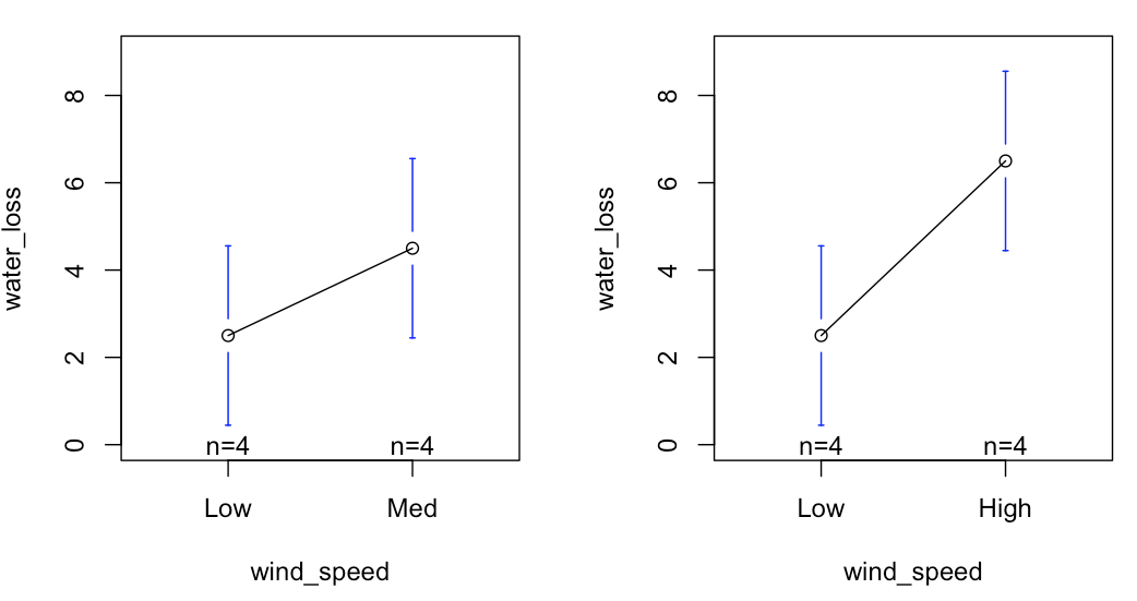
We can plot these data as R sees them in the lm analysis, as shown in the right. The regression line passes through the mean of each group. Consequently:

the Y-intercept is the mean of the "Low" 'wind_speed', and;
the slopes of the lines are DIFFERENCES BETWEEN means (Left = "Low" vs. "Med"; Right = "Low" vs. "High")

By setting up each level of the predictor as a contrast to the defined reference, then the slopes are simply the differences between the reference and the other categorical levels. In this case the slopes are IDENTICAL to the differences because the levels are exactly one unit apart on the x-axis. So, for a one-unit change in wind speed category, we see the associated changes in water loss.

In short, the Y-intercept is the mean of the reference category, and the other regression coefficients become "contrasts" from the reference mean.

Notice that R uses the variable name as a prefix for the identifier of each level of the variable - so the "Med" level of the 'wind_speed' variables becomes "wind_speedMed".

Do the coefficient estimates match what you expected based on the graph?

Yes - Low wind speed has the lowest mean water loss, and is ~2 units of water loss below the water loss when wind speed is Med.
To calculate the mean water loss values for "Med" and "High" wind speed, we simply add the "Intercept" value to each estimate. So, the mean water loss for "Med" = 2.5 + 2.0 = 4.5

There are approaches for considering which specific groups differ from one another given a significant overall P-value from the ANOVA - such as we have here. We will explore these later - but be mindful that the t-test for each coefficient presented in this output from the lm tests the null hypotheses that:

mean water loss at "Low" wind speed ("Intercept") = zero;
mean water loss at "Med" wind speed (wind_speedMed") = mean water loss at "Low" wind speed ("Intercept");
mean water loss at "High" wind speed (wind_speedHigh") = mean water loss at "Low" wind speed ("Intercept").

These are not necessarily the null hypotheses that make the most biological sense!

5.3 One-way ANOVA - more complex data

Having analysed an artificially simplified data set, now let's apply the same R code to a real example.

Import PlantGrowth.csv, and View it.

PlantGrowth <- read.csv("Data/PlantGrowth.csv", header = TRUE)

Effects of pruning roots or shoots on plant growth

A group of researchers were investigating whether they could accelerate plant growth, and conducted an experiment in which they applied five different intensities of pruning to either the roots or the shoots (leaves and branches):

two intensities of shoot pruning ('n25' and 'n50');
two intensities of root pruning ('r10' and 'r5'), and;
a 'control' that was not pruned.

They then measured the response to these treatments as the change in total biomass of the plant between the date on which the pruning treatments were applied, and three weeks after pruning.

ANOVA is a suitable way to analyse these data because:

there is a predictor variable, "pruning", with five levels ('n25', 'n50', 'r5', 'r10', 'control'), and;
within each level of the predictor, multiple measurements of a continuous response variable ("biomass") have been taken.

click for plants

First, we will plot the data. Visual inspection of the data is critical to thinking about whether the results of the statistical analysis are reliable. In Practical 3 we showed you how plotting the mean +/- SE can give you a preview of whether you expect a t-test to reject your null hypothesis of no difference. We can use the same approach for categorical predictors in ANOVA.

Use the "gplots" package (you may need to install using install.packages) and plotmeans function to graph the means of each level of "pruning" with their upper and lower 95% confidence intervals (calculated as .95*SE):

install.packages("gplots")
library(gplots)  ## Load the package "gplots"

## Plot mean biomass, with error bars, across different levels of pruning
plotmeans(PlantGrowth$biomass ~ PlantGrowth$pruning, connect = FALSE)

What does this graphic tell you about the effect of 'pruning' on 'biomass'?

The average 'biomass' is not the same for each level of 'pruning'.

What do the error bars tell us about the the effects of pruning on plant biomass?

'Pruning' is not the only thing affecting 'biomass'.
There is some unexplained variation in 'biomass' within each category of 'pruning'.

Now statistically analyse the data:

fit <- lm(biomass ~ pruning, data=PlantGrowth) ## Fit a linear model between biomass and pruning
anova(fit) ## Generate an ANOVA table

Does 'pruning' significantly affect 'biomass'?

Yes.
Within the ANOVA table, there is a large F-statistic and a small P-value for 'pruning'.

Which aspect of the ANOVA table tells you that 'pruning' is not the only thing affecting 'biomass'?

The residual variance (Residual Mean Sq) is not zero.

Now look at the regression coefficients. Because these are stored within the R object "fit", along with the other results of fitting the linear model, we can extract them and store them under a new name:

beta <- fit$coefficients  ## Extract the regression coefficients
beta

Which level of our 'pruning' variable was designated as the "Intercept"? Why? How can you interpret this intercept for an ANOVA?

'control' (which is quite convenient)!
Alphabetically, "c" comes before "n" and "r".

To see how R has actually coded the dummy variables, we can look at the "model matrix" of "fit":

model.matrix(fit)

Think of dummy variables as switches. Values of "1" indicate when a coefficient is switched on and values of 0 indicate when a coefficient is switched off. Importantly, the intercept (mean for the reference level) is always switched on. The other dummy variables are used to switch on (and off) the difference between the reference level mean and the mean of each other levels.

The regression coefficients, and t-tests on them, are generated in R using the summary command.

summary(fit)

The first P-value is for the reference level, in this case the "control" level of 'pruning'.

This P-value helps us decide whether to reject the null hypothesis that this value is zero. Put another way, it answers this question:

"Is the 'control' significantly different from zero?"

Should we accept or reject this null hypothesis? Biologically, what does it tell us?

Reject - the t-value is very large, and the P-value is very small.
This tells us that the plants that had not been pruned did grow (increase biomass) during the experiment.

What null hypothesis is assessed by the other t-tests reported in this output, and do you think that these are biologically sensible hypotheses for this experiment?

The mean of the each pruning level (i.e. each pruning treatment) is the same as the "Intercept" (mean of the "control")
This is a biologically sensible hypothesis for this experiment. Each of the other levels of 'pruning' are some treatment we have imposed, and so it is sensible to determine whether that treatment affected plant biomass, and an unpruned control is a sensible reference for this test.

Which 'pruning' treatment(s) affected biomass, relative to the unpruned control?

All of them - although the t-values are larger for the two root treatments than the two shoot treatments

5.4 Diagnostics

As for any regression technique involving F-statistics, the assumptions of normally-distributed residuals and constant residual variance must be verified for your data. If the assumptions are violated, we cannot be sure that the P-values are reliable!

5.4.1 Normally-distributed residuals

Check this assumption:

hist(fit$residuals)    ## Do the residuals look normal?
qqnorm(fit$residuals)  ## Does the qqplot look straight?
qqline(fit$residuals)  ## Add a straight line for comparison.

Is there any convincing evidence that the residuals are not normally distributed (Gaussian)?

No - the majority of dots form a straight line, matching the theoretical predictions from the normal distribution.

5.4.2 Constant residual variance

Let's now look at the second assumption in detail.

The F-statistic tells us whether the mean changes across the levels of an explanatory variable provided the residual (error) variance is the same within each level of the explanatory variables. If the residual variance is constant, a large F-statistic can happen only if the five means are not the same.

This is called "the assumption of constant variance", and it is fundamental to the logic of ANOVA. Without it, we cannot interpret F-statistics.

For example, we assume the error variance is the same within each category of 'pruning'. The assumption is evident in the ANOVA table itself; there is a single estimate for the error variance, called the "Error Mean Square", that is our best estimate of the constant error variance. It is based on all the data taken together across all levels of 'pruning'.

Test the assumption using Bartlett's statistical test:

plot(fit$fitted, fit$residuals)
bartlett.test(biomass ~ pruning, data = PlantGrowth)

This graphic is a plot of "fitted values" (values predicted by the linear model) against the "residuals" (the part not explained by the model). Look at the degree of vertical scatter. There should be no hint of a consistent trend as you scan from left to right. If there is no trend, then the assumption of "constant variance" holds.

Bartlett's statistical test for "homogeneity of variances" gives us an objective guide; if the P-value is small, then the within-group variances are not the same among the groups and we have a problem.

Based on the Bartlett test, is the residual variance constant across groups?

Yes. The P-value is large so we do not reject the null hypothesis that the residual variance is constant across groups.

5.4.3 Using `plot` to view diagnostic plots

The plot function can be applied to the output of any model fit, and automatically adapts its response according to the object supplied. For example, if an object was generated by either lm or glm, then you will see four consecutive diagnostic plots (the first two you have already generated above):

"fitted values" versus "residuals";
"qqnorm" graph;
"fitted values" versus "standardised residuals", and;
"residuals" versus "leverage".

These are obtained progressively by pressing the "enter" key repeatedly from the "Console" (bottom left) panel of RStudio, after you run the command:

plot(fit)

NB: the "leverage" plot returns an error for this dataset; you don't have to worry about that for now

Why bother looking at these graphical diagnostic images?

To satisfy the assumptions of ANOVA; the diagnostics need to be OK before we can trust the P-values printed in the ANOVA table.

5.4.4 Post hoc multiple comparisons

So far our anova() summary provided the omnibus test (i.e. overall test) of the null hypothesis that all treatments have the same mean. Then, the summary of the linear model gave us "treatment contrasts" where each pruning treatment was compared to the mean of the control using t-tests. What we do not yet know is how the "non control" treatments differ from each other. For this we need to take a separate additional ("post hoc") step - a Tukey test!. Luckily, this is easy in R!

TukeyHSD(aov(fit))

This provides tests on all pairwise combinations of our pruning treatments. Because there are five treatments there are 4+3+2+1 = 10 pairwise combinations (excluding each treatment being compared with itself). For each combination, a difference is provided along with upper and lower 95% confidence intervals and p-values. You may notice that the p-values are significant for differences that have confidence intervals that do not overlap zero. Also, the p-values for the comparisons with the control treatment are higher than they were in the linear model summary. This is because the Tukey test accounts for the additional statistical tests that are being undertaken. This is desirable because it reduces the probability of type I error (i.e. falsely finding differences that don't exist).

5.5 Two-way ANOVA - now we're getting serious!

Effects of coral bleaching on fish diversity in the northern and southern Great Barrier Reef (GBR)

A team of marine biologists undertook fish surveys on a number of healthy and bleached reefs in the northern and southern parts of the GBR. They calculated diversity from the raw survey data using the Shannon Index of diversity (a commonly used metric of diversity that accounts for the relative abundance of each species). The categorical predictor variables are simply:

reef

"healthy";
"bleached".

region

"north";
"south".

Two-way ANOVA is a suitable way to analyse these data because:

there are two predictor variables and the design is a full factorial design such that each combination of the two variables is represented (i.e. health+north, healthy+south, bleached+north and bleached+south).
within each combination of the predictors, multiple measurements of a continuous response variable ("shannon_diversity") have been taken.

Import the data, fish_data.csv.

fish_data<-read.csv("Data/fish_data.csv")

How is R treating each variable?

summary(fish_data)

R is treating our two categorical predictor variables as characters. This is ok, but when we start fitting models we are again at the mercy of R's arbitrary decisions about which levels are the reference levels for each predictor variable. We can take control of this situation. First, let's use the super helpful table() function to see what categories are in each predictor.

table(fish_data$reef, fish_data$region)

So now we can see the names of the different categories. This helpful table also tells us that there are 15 observations of fish diversity in each of the four treatment combinations!

For "region" it doesn't really matter which order of levels we use. But for reef, it makes sense to tell R to treat "healthy" as the REFERENCE LEVEL.

## re-define the reef variable specifying the order of the levels that we want
fish_data$reef <- factor(fish_data$reef, levels=c("healthy", "bleached"))

Before we do statistical analyses, PLOT THE DATA to see what we are working with. Here I use ggplot() (from the tidyverse package that you already installed) to plot a box and whisker plot coloured by treatment. Don't worry about the strange syntax - ggplot() takes some getting used to but it is a very powerful way to visualise data very quickly. We will give you the basics of ggplot() later in the course. We use it here to expose you to some of the amazing plotting options at your disposal in R.

library(tidyverse)
ggplot(fish_data, aes(y=shannon_diversity, x=region, fill=reef))+
  geom_boxplot() +
  geom_point(position=position_jitterdodge(jitter.width=0.25), alpha = 0.3)

So at first glance our data look normally distributed (the boxes in the box and whisker plot are more or less symmetrical). Each box is also roughly the same size, so we are likely meeting our assumption of constant variance. Intriguingly, we can also see that the effect of bleaching on fish diversity appears to be different in the northern region than it is in the south!!! In other words, the effect of bleaching DEPENDS ON region, so we almost certainly need to include an interaction in our model! We do this by including " + reef:region" in the model formula.

fish_mod <- lm(shannon_diversity ~ reef + region + reef:region, fish_data)

plot(fish_mod$fitted.values, fish_mod$residuals) ## Plot the residuals against the fitted values to assess constant variance
qqnorm(fish_mod$residuals)   ## Check normality of residuals
qqline(fish_mod$residuals)   ## Plot expected fit for comparison

Is there any evidence that the residuals do not have a constant variance?

No. Our plot of residuals versus fitted values look fine, as we expected given our exploratory box and whisker plot. We meet the assumption of constant variance.

Is there any evidence that the residuals are not normally distributed (Gaussian)?

Again, No. The qqplot looks great and the residuals follow the theoretical expectation (diagonal line).

5.5.1 Look at the results

anova(fish_mod) ## ANOVA summary first

As expected, the interaction is significant. Let's visualise the means of each treatment combination to make sense of it.

## we can plot interactions using plotmeans, like this:
plotmeans(shannon_diversity ~ interaction(reef, region), 
          data = fish_data, connect = list(1:2,3:4), ylim = c(1.4, 3.1))
## we tell plotmeans to connect up the first 2 points with a line 
## and the last two points with a line
## these lines represent the slope of the bleaching effect in each region!!!

Now we are ready to interpret the coefficients from the summary of the model.

summary(fish_mod)

Looking at the plot we just made, and thinking back to the lecture, can you interpret the four coefficients?

The intercept is the mean fish diversity for healthy reefs in the north. We know this because we manually forced R to use "healthy" as our reference level for the reef variable, and because we let R choose the reference level alphabetically for region (north comes before south). Try and work out the rest yourself. Remember from the lecture, interaction terms are "slope adjusters". We will walk you through this as a group.

As with one-way ANOVA, we can conduct post hoc multiple comparisons with two-way ANOVA. Below we use the same TukeyHSD() function that we used previously. We also introduce the more flexible emmeans() function from the emmeans package. The results are almost identical in this case, which is reassuring. As you will see in coming weeks, the emmeans() function can be used in a great variety of situations, and on models with non-normal error distributions. For now, just enjoy meeting your new friend, emmeans.

## pairwise Tukey test
TukeyHSD(aov(fish_mod))

## install the package first
install.packages("emmeans")
library(emmeans)
emmeans(fish_mod, specs = pairwise ~ reef:region)

5.6 Do it on your own

The restoration ecologist dressed in double denim during the implementation of the seedling experiment

A restoration ecologist named "John" conducted an experiment to examine the effects of shading and watering on the performance (biomass (kg)) of seedlings of an ecologically important tree species Eucalyptus tereticornis. The species is used a lot in restoration of koala habitat as it is a preferred koala food tree species.

Step 1. Read in the data. On your own, try and look at a summary of the data. Work out what the variables are, what the categories of each variable are, and how R is treating each variable.

seedling_data<-read.csv("Data/seedling_data.csv") ## read in the data

Step 2. Plot the data! Does it look like ANOVA will be a suitable tool to analyse this dataset? Is there evidence that an interaction is required?

Step 3. Think about how R will treat each variable if left to its own devices. If you need to manually tell R the levels of a variable, do this now. If it looks ok, proceed.

Step 4. Fit a linear model.

Step 5. Check the diagnostic plots before proceeding to statistical inference (i.e. before looking at anova tables and model summaries).

Step 6. If the assumptions of linear modelling are being met, proceed to inference. First look at an anova() table, then a summary().

Step 7. Compare the model summary to a plot and try and work out what each coefficient estimate represents.

Step 8. Try and test pairwise differences using a post hoc multiple comparison procedure.

Step 9. Finally, what do these results tell us about the performance of E. tereticornis in different restoration contexts?

5.7 List of useful functions

Here are a few useful functions that you used today.

gplots::plotmeans; ggplot2::ggplot

Check assumption of normally distributed residuals
hist; qqnorm; qqline

Post hoc multiple comparisons
TukeyHSD; emmeans::emmeans