Practical 1 Getting started with R

Why learn R?
R is a professional statistical package, it is:
- The tool of choice for most professional biologists and scientists;
- FREE;
- The most up-to-date, all-purpose statistics package available: a huge group of users constantly up-date and add resources to R;
- Immensely powerful, you can use it to:
- manipulate and organise data;
- run statistical models, from simple to highly complex ones;
- handle multiple data sets simultaneously;
- produce beautiful graphics, and;
- build and run simulation models to understand and quantify biological dynamics.
Whatever your career path, R-literacy is an important skill to have on your CV!
1.1 Installing R and RStudio
By now you should have installed R and RStudio onto your personal computer. We repeat the instructions here in case you need to re-install or update in the future. Install R for your operating system (Windows, macOS, or Linux).
An icon will appear on your desktop, and a collection of folders (directories) will also have appeared at the location you specified during the installation. The CRAN (COMPREHENSIVE R NETWORK) website contains a lot of useful information about R: manuals, documentation, FAQs, access to the R-Help archives, add-on modules for download, and more. The Internet is also pretty helpful!!!
When you first install R it comes with the "Base Package" that includes many essential functions. This base has been built on and extended by many practitioners, and we will use other packages to support our analyses. In coming weeks, we'll show you how to install and load these packages.
R is a very "old school" command-line driven application, but there are many wrappers available that drag R into the 21st century, and provide a more user-friendly interface. We will use RStudio, one of the most popular interfaces. Only install this AFTER you have installed R.
1.2 R Projects (inside RStudio)
Biologists, ecologists and conservation scientists who routinely analyse data are often working on more than one analysis at a time. RStudio lets us make a "mini universe" on our computer for each specific project we are working on. These are called "R projects". By now you should have watched the instructional video on how to make an R project for CONS7008, complete with all of the data files we will use in this prac series. How convenient!
Navigate to your CONS7008 R Project and click on the "CONS7008 R Project.Rproj" file (depending on your computer you may not see the ".Rproj" file extension). RStudio should open automatically (it might take a little while, be patient). In the lower right panel, click on "Files" and then click on the little cube with "R" on it (to the very right-hand side). You will notice that you are "inside" the CONS7008 R Project folder. This will be the same on everyone's computer which is convenient because now we don't have to worry about telling R where we are on our specific computers (e.g. "/Desktop/Johns_crap/"). Instead, when we are inside this mini universe, R knows where to find files that we want to import, or were to put stuff that we want to output (e.g. nice figures!).
1.3 A quick reminder about file paths
We use code to tell R where our data files are so we can use them, and where we want R to save outputs. This is where file paths come in. A file path is simply the directions to a specific file. You can think of it as giving someone directions to a room in a house - you might say 'go to the second floor, then find the third door on the left'. When you set up your R project, you created a folder called 'Data', this is where you (hopefully) put all the data files. So, if we want to analyse our 'beetle_data', we need to tell R, go to the 'Data' folder, and find the file called 'beetle_data.csv'. In R code this is simply read.csv("Data/beetle_data.csv"). So when you see this kind of code in the activities below, you will understand what is happening.
1.3.1 Starting a fresh R script
The upper left panel of RStudio is where you write your R code into script files that can be saved. To start a new file, click the icon resembling a white page with a green + symbol in top left-hand corner of the script panel.
Press File -> Save. Rename the file "Prac 1 R script.R" and save it inside the "R scripts" folder. Now we are ready to do some REAL R programming!
You type or paste commands into R scripts, edit them, and pipe them into R by clicking the "Run" button; it will run the command at which the cursor is currently positioned. If you want to run several commands consecutively, highlight them all, and then click "Run". There are also helpful keyboard shortcuts that make it easier to send commands to R. For Windows use Ctrl+Enter and for a Mac use Cmd+Return.
You can have multiple different R script files open at once but for now let's keep it nice and simple with a single R script.
1.3.2 Navigating RStudio
Now that you are in RStudio, orient yourself to how it is laid out.
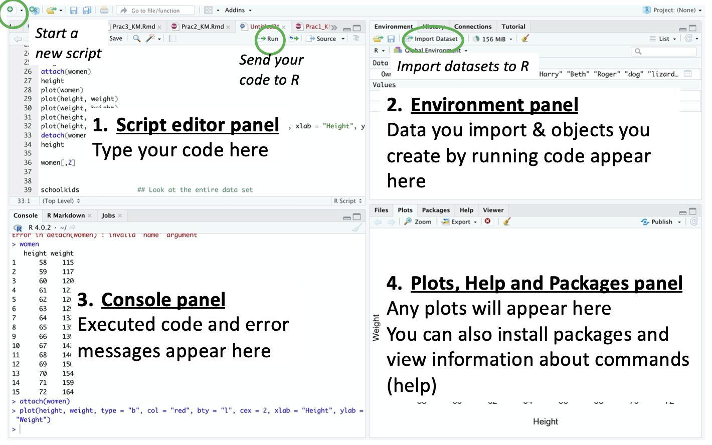
The R console is in the bottom left hand panel. Think of this as the brain that does all of the work. As you will see below, we generally don't type directly into the R console but it is possible (you won't break R!). Graphical output from R goes to the bottom right hand panel - that panel also has a tab to get information about functions ("Help") and a tab to manage the installed "Packages". The upper right panel shows your R Environment. This is where data objects and functions appear after you import or define them - this probably won't make sense at this stage, so don't worry about this yet.
Throughout this practical manual, R code will be presented in grey boxes (as below). You can copy the code by clicking the button at the top right corner of the box. Paste the code into your R script in RStudio, and then execute the commands.
1.4 Getting help
You can get information in R about any command by typing ? followed by the name of command you want help on.
Try running this command:
What happened? Did R do anything
You should have seen the code appear in the bottom left panel "Console", and information about the "with" command appear in the "Help" tab in the bottom right panel
When R responds to the ?, it usually displays an information page that gives example scripts at the bottom. You can cut and paste these scripts straight into the script editor, execute them, and see how they work. Another useful trick is to type example(command) where "command" is the name of the R command that you are trying to learn more about.
You can also "Google" your problems; just type "R" followed by your query. Problems with R are extensively discussed on Internet forums, so there is an extremely high chance that your problem has already been discussed and resolved.
And then there's AI. For experienced R users, AI is proving extremely useful (environmental and ethical considerations aside). It increases the efficiency and "elegance" of our code (by elegance I mean how wonderfully simple the code is to do a specific task). For beginners, we are still working out the best ways to use AI to teach coding so that you actually learn how to code. One major skill will be learning how to pose questions to AI so that you get correct and useful advice. We can also ask AI to explain what each line of code is doing, which should theoretically be a great way to learn. The problem is that AI tools don't always provide the best advice, especially if you don't quite know what details to include in the question.
1.5 Using R as a calculator
Copy the code below into your R script. Then "run" these commands and observe their effects:
1 + 2 ## Add 1 and 2
sqrt(1 + 2)  ## Take the square root of the sum of 1 and 2
x <- (48 + 34)/5.5  ## Make an R object "x" to store the result of adding 48 and 35, and dividing by 5.5
x   ## show the result in the console
Some tips on coding:
The
<-tells R "run the commands at the base (-) of the arrow and store the output as an object with the name pointed to by the arrow (<)". If you do not supply the arrow and a name, the output will appear in the console, but will not be saved in your R environment.Anything you type into R after the hash symbol (#) is ignored - this is useful for adding notes on your code. Annotate your code to tell yourself what it is doing to help you remember for future use. Any code you share with others (whether for assessment or as a collaboration) should be well annotated so the purpose of each line of code is clear.
R is case and font sensitive. For example, "Height", "HEIGHT", and "height" are completely different things. So take care when typing commands.
What is the answer to: (9 + 3.3)/(10.1 - 4)?
2.0163934
1.6 Vectors, classes, and some basic operations
R has a concatenate command: c(). Concatenate means "join together as a sequence", and such sequences are called "vectors". The stuff inside the brackets, separated by commas, is concatenated.
To pick and choose stuff within a vector, use [] as demonstrated below. Try this:
stuff <- c(6, "elephant", 4.5, 1, "cat", "elephant", 4.5)   ## Create a vector of "stuff" with numbers and characters
stuff                ## Show stuff in the R console
stuff[1]             ## Show the first element of stuff. Note the "" around the 6 - R has not recognised 6 as a number
class(stuff)         ## What type of class is "stuff"? Everything in "stuff" is recognised as a character
stuff[1] + stuff[4]  ## Error message because "6" and "1" are not recognised as numbers
stuff[2:4] ## The 2nd, 3rd, 4th elements of "stuff"Challenge: Write the code to make a new vector named "friends", concatenating the first names of your five closest friends (in no particular order!). Show the person next to you JUST the name of your third friend.
1.6.1 Changing between classes
Even though we might include a combination of text and numbers in a vector, the vector itself can only be one class. Because "cat" and "elephant" were in the "stuff" vector, "stuff" was recognised as a character vector, hence the "" around ALL elements. The code stuff[1] + stuff[4] looks like 1 + 6 to us, but to R it might as well have been "Rosalind" + "Barbara".
It is possible to change between classes. Here we create a new version of "stuff" that is numeric. We creatively name it "stuffNumeric":
stuffNumeric <- as.numeric(stuff)         ## There were warnings because "cat" and "elephant" can't be converted to numbers
class(stuffNumeric)                       ## Now it's a numeric vector!
stuffNumeric                              ## See the NAs where "cat" and "elephant" were? R has removed them because it couldn't convert them

stuffNumeric[1] + stuffNumeric[4]         ## Now this works as desired! 1 + 6 = 7
There are other classes too. A "factor" is a class used by R to deal with categorical variables in statistical models. Factors assign each unique value in a vector to a "level". R then orders these levels numerically and alphabetically. Let's explore the behaviour of factors using the "stuff" example again.
The factor is similar to "stuff", but now there are levels. Notice how the levels are ordered - numerically then alphabetically. Notice also that there is only one level for "elephant", even though there are two "elephant" values in "stuff". So levels identify the unique categories in a factor and give them an order.
Now try and convert stuffFactor to numeric:
stuffNumeric2 <- as.numeric(stuffFactor)  ## No warnings! Why?
stuffNumeric2                             ## This is now a vector of integers; everything has changed - these numbers are the ORDER that each of our original "stuff" appeared in when we converted to a factor.
What is going on with "stuffNumeric2"?
The numbers are the "levels" of "stuffFactor", rather than the actual values (6, 4.5, 1) from the stuffFactor vector. 4.5 is no longer 4.5, but the 2nd level of stuffFactor. Don't worry if this is super confusing. All you need to know at this stage is that factors are another class of vector that R uses. They start to make sense the more we use them.
In summary, classes are important and it is often necessary to switch between them, particularly for analysing data (e.g., to test for a difference between a "Treatment" and "Control" we need R to know that these are two levels of a factor, not characters). Be careful when changing class, particularly when changing from a factor to a numeric class.
1.7 Data matrices
Most of our work will involve data sets with more than one variable. For example, we might be working with an explanatory variable and a response variable.
Let's make some new data vectors, with the same length (i.e., the same number of elements):
Owners <- c("Sally", "Harry", "Beth", "Roger") ## Vector of four people's names
Pets <- c("dog", "lizard", "bird", "cat")      ## Vector of the type of pet each person has
Now let's combine these two vectors into one "matrix", and look at it:
OwnersPets <- cbind(Owners, Pets)  ## cbind concatenates these two vectors as columns
OwnersPets        ## Have a look at it
str(OwnersPets)   ## Check the class - here we've used "str" which is useful when you have multiple variables, or columns in your data
dim(OwnersPets)   ## the command "dim" returns the dimensions (number of rows and columns) of our object
What are the dimensions of the matrix "OwnersPets"? Is this what you expected it to be?
4 2; that is, four rows and two columns
cbind has joined the two vectors together to form a "matrix". In R, we can work with vectors, matrices, or "dataframes". These are similar, but have slightly different properties, and respond to different commands. This is useful to know, as sometimes the reason your code isn't working is because R thinks your data is in a different format to what you think it is (just like you saw with data classes).
We can alternatively create a dataframe using data.frame:
OwnersPets.df<- data.frame(Owners, Pets)    ## add the vectors to a dataframe
OwnersPets.df         ## Have a look at it
str(OwnersPets.df)    ## Check the structure
How does the structure of "OwnersPets" differ from "OwnersPets.df"?
"OwnersPets" is a list of 1:4 and 1:2 characters, while "OwnersPets.df" is arranged as four rows ("obs." or observations) and two columns (or variables)
1.8 Importing your own data into R
More often than not we import data into R rather than entering it into our R code like the "OwnersPets" matrix above. Data is typically stored in spreadsheets like you have probably used before in MS Excel. A spreadsheet must be in the right format before it can be imported into R. Specifically:
- The data must be in "row/column" format, i.e.:
- rectangular;
- each column holds a separate variable (e.g. "Height"), and;
- each row holds data from a separate object.
- Column names should be one word each, or multiple words separated by "_" (e.g. "wing_length") because R struggles with spaces in column names.
- There must be nothing in the spreadsheet but data (e.g., no extra notes, graphs, colour-coding etc). For this reason, we often store data as csv files because this file type doesn't support shading, colours and other fancy formats.
To explore dataframes further, let's import the csv file called zebrafish.csv into R. This file is located in the "Data" subfolder within our CONS7008 R Project, so we can easily import the data like this:
Why did we include "Data/" in the name of the csv file?
R needs to know where to find things. All of the .csv files for this course are stored in the "Data" subfolder within our R Project, so we need to tell R to get "zebrafish.csv" from inside the "Data" folder.
Check that your data is now imported by typing these commands:
zebrafish               ## Look at the entire data set
names(zebrafish)        ## List the variables (the column names)
head(zebrafish, n = 4)  ## Look at the first 4 rows of the data
tail(zebrafish, n = 4)  ## Look at the last 4 rows of the data
dim(zebrafish)          ## How many rows and columns are there?
What is the "zebrafish" data? How many variables (columns) and objects (rows)? What are the variables?
dim() will tell you that there are 482 rows by 10 columns; you can see the column labels when the object is called (i.e., you just run the object name), via the names() command, the head() or tail() commands.
1.9 Dataframes and viewing data
We can access columns in a dataframe in a few different ways.
zebrafish$TotalLength ## the values in the TotalLength column
zebrafish$TailDepth ## the values in the TotalDepth column

TailDepth ## You will get an error

with(zebrafish, TailDepth) ## the values in the TotalDepth column (same outcome as above)
What was the purpose of using with?
with tells R that "zebrafish" is the dataframe we are using, such that we could refer to 'TailDepth' and R knew where to access it from.What does the "$" do?
This tells R that the TailDepth variable can be accessed in the zebrafish dataframe. Try running the code: zebrafish[, 7] - what is it equivalent to?
One of the first steps researchers take when looking at a dataset for the first time is some basic visualisations. Often we are interested in how individual variables are distributed (are they normal, skewed, other?) and how pairs of variables might be related to one another. To visualise distributions we can use a simple histogram and to visualise relationships we can use scatterplots. Let's try this quickly now using the zebrafish data, but we will dig a bit deeper into plotting later in this prac.
hist(zebrafish$SwimSpeed) ## a hisogram of the "SwimSpeed" variable

hist(zebrafish$TotalLength) ## a histogram of the "TotalLength" variable

plot(zebrafish$SwimSpeed ~ zebrafish$TotalLength) ## a scatterplot with SwimSpeed on the Y-axis and TotalLength on the X-axis

with(zebrafish, plot(SwimSpeed ~ TotalLength, col = "tomato")) ## the same plot, but with red points this time!
## Notice how we used "with" in this example instead of using the $ to tell R which dataframe the variables are in
What does "col" tell R to do?
type "??col" into your code and run it. Click on graphics::par to see all of the graphical parameters
1.10 Classes within dataframes
Above, you saw that all elements of a vector were treated as the same class (e.g., factor, numeric, character). In dataframes, this applies to each column.
If R encounters a non-numeric character within a column it treats the entire column as a categorical variable (i.e., as a non-numeric variable), even if all other entries are numbers. Therefore, if you have accidentally typed a non-numeric character (even an accidental "space") into your data column, you have to go back to the data file and fix it before importing the data back into R.
As with vectors, it is possible to change the class of columns. You can use the "structure" function, str, to identify the class of each column.
In the "zebrafish" dataframe, 'sex_nr' is a categorical variable for "sex", but R does not recognise that because sex has been coded as numbers: 1 and 2. You need to tell R to treat them as categories using the as.factor function.
Try this:
The variable 'sex_nr' is now a categorical variable (a factor) within "zebrafish".
Even though it is more typing, it is often safest to use $ to ensure that R is very clear about what variable you are asking it to act on.
1.11 Picking and choosing parts of a data set
Sometimes you will want to select (or identify) parts of a dataset. Above, we used stuff[1] to get the first element of the "stuff" vector. For dataframes (which have rows and columns, i.e., they are 2-dimensional, not 1-dimensional), we need two arguments. Again, we use the [], but slightly differently.
Copy the below code and run each line, and deduce what each command does.
zebrafish[2, 4]
zebrafish[, 2]
zebrafish[2, ]
zebrafish[, 1:3]
zebrafish[zebrafish$TotalLength > 30, ]
with(zebrafish, zebrafish[sex_nr == 1, ])
zebrafish$sex_nr
zebrafish[, "sex_nr"]
The > and == commands are basically TRUE/FALSE questions (referred to a "logical arguments") that we can use to select specific rows in the dataframe.
Hence, when subsetting the data like this: zebrafish[zebrafish$TotalLength > 30, ], R shows all of the rows where zebrafish$TotalLength > 30 is TRUE.
How many "zebrafish" have a 'TotalLength' less than 20? Of these, what is the longest 'TotalLength'?
6; 19.8
NB: == and = are different. == is a TRUE/FALSE question, whereas = tells R to make the values to the left and right of the "=" the same.
Picking and choosing parts of a data set is relatively easy if you remember a few basic rules:
DataSet[RowNumbers, ColumnNumbers]
DataSet$ColumnName
DataSet[RowNumbers, ]$ColumnName
DataSet[RowNumbers, "ColumnNames"]
What would these command produce?
DataSet[, 1:2]
DataSet[1, ]
DataSet[1:5, ]$Col1Name
DataSet[1:5, "Col1Name"]
The first two columns, ALL rows.
The first row, ALL columns.
The first five rows, and the first column (named "Col1Name").
Exactly the same as the one before!
1.12 Graphing data
The graphics in base R are customisable, and capable of anything you are likely to want (given enough time, effort, and patience). We will show you quite a few ways to plot data in this course - there is a wealth of expertise in plotting available via the R community on the Internet.
To get started, run the code below, and see how it changes the plots.
plot(zebrafish$SwimSpeed ~ zebrafish$TotalLength, type = "n",  ## Set up a blank graph with axes (type = "n" makes the plot blank)
     xlab = "Fish length (mm)", ylab = "Fish swimming speed")  ## Add axis labels

with(zebrafish, points(SwimSpeed[sex_nr == 1] ~ TotalLength[sex_nr == 1], col = "goldenrod")) ## Insert gold points for the 1st sex
with(zebrafish, points(SwimSpeed[sex_nr == 2] ~ TotalLength[sex_nr == 2], col = "tomato"))  ## Insert red points for the 2nd sex

## now make new plots of the same relationship, but we will tweak some graphical parameters each time
plot(zebrafish$SwimSpeed ~ zebrafish$TotalLength, bty = "l")          ## Remove the surrounding box type

plot(zebrafish$SwimSpeed ~ zebrafish$TotalLength, xlab = "Fish length (mm)",
     ylab = "Fish swimming speed", cex.axis = 1.5, cex.lab = 1.5)  ## The "cex" (= character expand) command controls the sizes of characters

## We can even look a a bunch of pairwise plots at once using a scatterplot matrix
with(zebrafish, pairs(SwimSpeed ~ TotalLength + TailDepth + BodyDepth   + HeadLength, upper.panel = panel.smooth))
The plot command has many subcommands, giving you finer control over the appearance (see ?par and ?plot for more details).
Is sex_nr 1 or 2 shown in red on the plot?
points(TotalLength[sex_nr == 2], SwimSpeed[sex_nr == 2], col = "red")
1.13 Installing and loading packages
Throughout these practicals, we will sometimes need to run commands that aren't available in R by default. We can make our own R functions to solve a task, but often someone else has already done that for us. People write functions and then compile them into packages for everyone to use. This is extremely helpful, and a large part of what makes R such a powerful tool.
Have a go at installing a package using the code below:
install.packages("praise") ## This installs the package onto your computer in your default 'library' You can also install a package using the buttons under the "Packages" tab in the bottom right panel of RStudio.
After you have installed the package, if you want to run a function that is contained in that package, you first have to load the package:
library(praise)  ## This command loads the 'praise' package
require(praise)  ## This also loads the 'praise' package
NB: library and require are identical commands, you might see both around, but they both just load packages.
Now try running the praise() function. I was "exquisite" - what are you?
If a package is installed on your computer, you can run a function without loading a package like this: praise::praise().
1.14 Saving and Tidying up
At any time (indeed frequently!) save your R script of commands and notes.
When you are finished with them, it is good practice to remove any variables you've created during the session from your R Environment. This can all save confusion with any further commands and objects you introduce later.
You can get rid of everything by typing:
Notice how everything disappeared from your Environment in the top right panel of RStudio?
This can be really helpful in some situations where R has gotten confused; for example, if you have created multiple dataframes that share variable names. Once you have done this though, you will need to go back and re-import the data, and re-run the code to create any R objects that you want to work with. This is why saving R scripts is so important! It saves all of the "instructions" for R and you can just run it again in a fresh session.
You can also use the "broom" button that you see at right-hand end of the icons above the Console, Environment and Plot panels of RStudio - that will delete everything in those panels.
1.15 List of useful functions
Here are a few useful functions that you learned today.
Classes
as.character; as.numeric; as.factor
Making/unmaking a dataframe the default to apply any future commands to
with
Data structure
head; tail; str; dim; names
Visualisation
hist; plot; pairs
Installing and loading packages
install.packages; library; require