Practical 7 Linear mixed-effects models
Analysis of covariance (ANCOVA) is a form of linear models in which there are both continuous and categorical predictor variables. It combines linear regression with analysis of variance (ANOVA). While there are many biological questions where both continuous and categorical predictor variables are of interest, one way in which ANCOVA is commonly used is when we want to control for the influence of one variable so we can interpret the other.
People who routinely use ANCOVA refer to the continuous predictors as "covariates", and refer to the categorical predictors as "groups".
ANCOVA can be used:
- When the categorical predictor is the focus of the study, adding a covariate to an ANOVA can reduce unexplained variation in the response variable, thereby increasing the power to detect differences among groups (i.e., an effect of the predictor variable of interest on the response);
- When the continuous predictor is the focus of the study, adjusting a linear regression model according to the levels of a categorical variable can provide greater insight into the effect of the continuous predictor, and how these intercepts and slopes differ among groups.
In this practical, we will explore three ANCOVA examples, and use a combination of statistical modelling and graphing techniques to assess model assumptions.
Considerations of ANCOVA
Beyond the usual assumptions of regression and ANOVA, our ability to interpret ANCOVA depends on two further considerations:
- Covariate values cover a similar range across groups
- Regression slopes are similar across groups.
If the first assumption is not met, it actually tells us that the two predictor variables are collinear, or confounded. In this case, ANCOVA might then fail to separate the effects of the two explanatory variables on the response variable in a similar way that you saw with confounded predictors in multiple regression in week 5. We will explore the consequences of violating this assumption in section 7.6.
If the second assumption is not met, you can still fit a linear model to the data, but cannot use a standard ANCOVA approach. Just as you learned in week 6 about interpreting main effects, when there is a significant interaction between explanatory variables, the interpretation becomes more complicated. In the case of a significant interaction between a covariate and a categorical predictor, the comparison of groups is more complicated as it has to be carried out separately at different values of the covariate. Even if you can't run a standard ANCOVA analysis due to varying slopes, discovering that your categorical predictor variable of interest has an interacting relationship with a continuous covariate might be a new and exciting biological insight that leads your research on to new pastures.
7.1 An example with data well-suited to ANCOVA
Effects of mating on longevity of male flies
A study of male vinegar flies (Drosophila melanogaster) was carried out to answer this question:
The researchers specifically predicted that the energetic requirements of sperm production, courtship, and mating would shorten lifespan, resulting in males that "live fast and die young".
Male flies were studied individually. The categorical predictor variable, 'Treatment', had five levels, differing in access to receptive females:
- "Alone": no female presented to the single male fly;
- "Virg1": a single virgin female presented to the single male fly;
- "Virg8": eight virgin females presented to the single male fly;
- "Mated1": a single already mated female presented to the single male fly;
- "Mated8": eight already mated females presented to the single male fly.
Because female D. melanogaster that have mated are able to store sperm, they remain unreceptive to males for some time. Thus, this study has two controls (no interaction with any flies: "Alone"); interactions with non-receptive females ("Mated1" and "Mated8"), which allow the researchers to clearly determine effects of mating (including sperm production and courtship) on survival, separate from any other factors associated with being present in a vial with females.
Size is known to affect longevity in D. melanogaster. Thorax length ('Thorax') of each male fly was also recorded as it is an easy to measure proxy for overall body size. Size is the continuous predictor in the analysis.
The longevity (number of days alive; 'Longevity') of each male fly was measured, and is the response variable.
This data presents the simplest scenario for ANCOVA as it involves just one of each type of variable.
The data are available in the file: DrosLongevity.csv.
DrosLongevity <- read.csv("DrosLongevity.csv", header=T)First, get a overview of the relationships between predictor and response variables by plotting the effect of thorax length ('Thorax') on longevity ('Longevity'), separately for each group (type of female) as follows:
## Make a list of the levels of the treatment
uTreatment <- unique(DrosLongevity$Treatment)

## Set up the axes
plot(DrosLongevity$Thorax, DrosLongevity$Longevity, type = "n")

## Add add data points separately "for" each female type
for(i in 1:length(uTreatment)){
  with(DrosLongevity, points(Thorax[Treatment == uTreatment[i]], Longevity[Treatment == uTreatment[i]],
  pch = i, col = i))
}

## Add a legend
legend("bottomright", legend = uTreatment, pch = 1:length(uTreatment), cex = 0.8, col = 1:5)
Do the values of 'Thorax' (the covariate) cover a similar range across the various groups?
Yes; for each group, the range of 'Thorax' on the x-axis is similar.
Does it matter? Why are we concerned about ranges?
If the range of the covariate is not the same across groups, the "covariate" and "groups" are collinear, or confounded, which would make it difficult to separate their effects on 'Longevity'.
Here, if we found a relationship, it would suggest that the researchers had not been successful in assigning males at random to each of the treatments. Rather, they had accidentally assigned larger males to one treatment, and smaller males to a different one. Luckily, they appear to have successfully assigned males at random!
Can you tell from this graph alone whether either of the two explanatory variables ("covariate" and "groups") have any significant effect upon longevity?
No. We need to fit the model with both factors before we can reject (or accept) the null hypotheses. For this many observations and treatments it is difficult to "see" the spread about treatment means to know how precisely the means are estimated.
However, patterns that we see here can help us to understand the results of the model when we have fit it. As was known before the experiment was conducted, larger flies do appear to live longer (trend from bottom left to top right of graph). The points corresponding to males given access to multiple virgin females ("Virg8") also seem be distributed lower on the y-axis, suggesting that mean longevity MIGHT change with levels of mating.
7.2 Regression modelling and diagnostics
The techniques of ANOVA can help us to decide whether the covariate ('Thorax') and/or groups ('Treatment') have any significant effect upon our dependent variable ('Longevity'). They can also help us decide whether the two explanatory variables interact in their effect on longevity.
In making these decisions, we use the sizes of the P-values in the ANOVA table as our guide. It is important, therefore, to have faith in the accuracy of those P-values. First, check the "diagnostics" of the data analysis.
model1 <- lm(Longevity ~ Thorax * Treatment, data=DrosLongevity) ## Fit the full model
plot(model1)  ## Check the diagnostics
Remember: The * tells R to "fit every possible combination of".
Does the "constant residual variance" assumption check out?
No. There is a tendency for vertical scatter (residual variance) to increase with the fitted value.
Does the "Gaussian residuals" assumption check out?
Yes. The qqplot is reasonably straight.
In order to improve the diagnostics, try log-transforming the response variable.
model2 <- lm(log(Longevity) ~ Thorax * Treatment, data=DrosLongevity)  ## Fit the full model with log(LONGEV)
plot(model2)   ## Check the diagnostics
Has the log-transformation improved the diagnostics?
Yes. The vertical scatter of the residuals seems less dependent on the fitted value.
The qqplot remains reasonably straight.
We are now in a position to look at the P-values and statistical significance with some confidence in their accuracy.
anova(model2)How should we interpret the interaction between 'Thorax' and 'Treatment'?
We accept the null hypothesis that the slope of thorax size on longevity is the same for all levels of treatment (i.e., parallel slopes).
This is great news! It certainly simplifies how we can interpret the "main effects" - if we had rejected the null hypothesis of parallel slopes, we could not interpret the average effect of different levels of mating, only the effects for flies of a specific size (i.e., for each level of the covariate).
The interaction between 'Thorax' and 'Treatment' is not significant. We can test a simpler model against our interaction model to determine if we can drop the interaction term without losing a significant amount of explanatory power using an anova test:
model3 <-  lm(log(Longevity) ~ Thorax + Treatment, data=DrosLongevity)   ## Fit a model WITHOUT the interaction term
anova(model2, model3)  ## We can compare the models to confirm that the interaction is not significant
anova(model3)  ## Observe the model results without the interaction term
What does our model comparison show us?
The F-value is small and the p-value is large, indicating that we cannot reject the null that the models explain similar amounts of variation in the data. Therefore, we can drop the interaction term and use the simpler model (model3) to analyse our data without any loss of information (you can revist Prac section 5.5 for a refresher on this idea)
Does 'Thorax' significantly affect the 'Longevity' of male flies?
Yes. The F-value for 'Thorax' is large and the P-value is small (<<0.05).
Does variation in access the number and/or type of female a male encounters affect his lifespan?
Yes. The large F-value and small P-value of the main effect of 'Treatment' allow us to reject the null hypothesis that average 'Longevity' is the same across all the treatment groups.
We can consider further the effects of each treatment level:
summary(model3) #inspect the beta coefficients and associated t-testsWhat does the Estimate for 'Thorax' tell us?
The estimate is positive, indicating that the slope of 'Lifespan' on 'Thorax' length is positive. Hence, 'Lifespan' increases with 'Thorax' size.
Does access to receptive females significantly shorten the lifespan of male flies? Remember: the "Virg1" and "Virg8" levels of 'Treatment' are the receptive females.
Yes.
The t-tests contrasting these to the baseline of "Alone" suggest we should reject the null hypothesis that 'Longevity' is the same: P-values for "TreatmentVirg1" and "TreatmentVirg8" are small (0.0247 and <<0.0001, respectively)
The beta estimates are both negative. This tells us that, relative to "Alone" flies, males with receptive females had shortened life spans.
7.3 Plotting regression lines for each group
In the last section, the interaction between 'Thorax' and 'Treatment' was non-significant; the groups share an identical relationship between the response variable ('Longevity') and the covariate ('Thorax'). That is, the regression line has the same slope for each group.
The following code generates an image that illustrates this interpretation of the data by plotting the regression slopes estimated from the analysis.
#First, re-create the previous graph (remembering to log-transform 'Longevity'):
plot(DrosLongevity$Thorax, log(DrosLongevity$Longevity), type = "n")
for(i in 1:length(uTreatment)){
  with(DrosLongevity, points(Thorax[Treatment == uTreatment[i]], log(Longevity[Treatment == uTreatment[i]]),
  pch = i, col = i))
}
legend("bottomright", legend = uTreatment, pch = 1:length(uTreatment), cex = 0.8, col = 1:5)

## Extract the regression coefficients from the reduced model
beta <- model3$coefficients

## Add lines based on the regression coefficients
abline(beta[1], beta[2], col = 1)
for(i in 3:6){abline(beta[1] + beta[i], beta[2], col = i - 1)}
Which aspect of this graph displays explicitly the lack of interaction between 'Treatment' and 'Thorax'?
All of the regression lines are parallel (i.e., they share the same slope).
Based on the graph alone, which treatment do you predict is mostly responsible for the significant 'Treatment' effect?
The "Virg8" group. Their dots are all low on the graph and the regression line is low and relatively isolated from the others, giving it a lower intercept on the y-axis.
Is your guess corroborated, in any way, by the t-tests for the regression coefficients (what R calls the 'Estimates')?
Yes! The regression coefficient for "TreatmentVirg8" was the most different to the reference baseline ("Alone"), and has an extremely small P-value.
Which statistic* reported by R in the anova output (anova(model3)) measures the variation among y-intercepts across groups?
The 'Mean Sq' for 'Treatment'.
7.4 Explaining noise
ANCOVA is sometimes employed in the interest of evaluating differences among groups: The covariate is included to account for "noise" in the data, and therefore reduce the standard error of the main effect of interest (the categorical predictor), and improve power to detect an effect.
When the covariate does indeed explain some of this noise (the "residual variance"), the differences among the groups are seen more clearly.
In the fly example, we might have only been interested in whether or not 'Treatment' affected 'Longevity' (i.e., we don't "care" about the effect of 'Thorax').
Fit the following regression model, involving 'Treatment' alone, and compare it to the previous model (model3) involving 'Treatment' and 'Thorax' together, as follows:
## Don't forget to log transform Longevity
model4 <- lm(log(Longevity) ~ Treatment, data=DrosLongevity)   ## Fit a model with only the categorical predictor
anova(model4)   ## View the results
anova(model3)   ## Recall results for covariate model for comparision
Does fitting size ('Thorax') as a covariate reduce noise? Compare the Residual Mean Sq: this is the best estimate for the magnitude of "unexplained noise" in the data.
Yes! The unexplained variance is ~1/2: 0.08 versus 0.04 when the covariate is included.
Does fitting size ('Thorax') as a covariate improve the power to detect an effect of 'Treatment'?.
Yes. The results suggest we should reject the null hypothesis (all treatments have the same mean 'Longevity') in both models. However, the our test statistic is substantially larger in the covariate model, and our confidence in rejecting the null is consequently greater.
7.5 An example where ANCOVA can go wrong
In the next two sections we will look at data in which our two predictors (categorical and continuous) do not vary independently, violating our first assumption of ANCOVA.
Within the context of ANCOVA, an easy way to judge independence between "groups" and the "covariate" is by looking at the extent of "range overlap".
We will now apply that technique to the FruitProd.csv data. Import the data, and View it.
FruitProd <- read.csv("FruitProd.csv", header = TRUE)Effects of grazing of fruit production
Research Aim: To evaluate whether fruit production in a plant species can be explained by:
- root diameter, and/or;
- grazing.
Response variable: "Fruit production" (a continuous response variable).
Explanatory variables:
- "Root: a continuous explanatory variable (being the diameter of the top of the rootstock), and;
- "Grazing": a categorical variable with 2 levels (groups):
- "Grazed", and;
- "Ungrazed" (protected by fences).
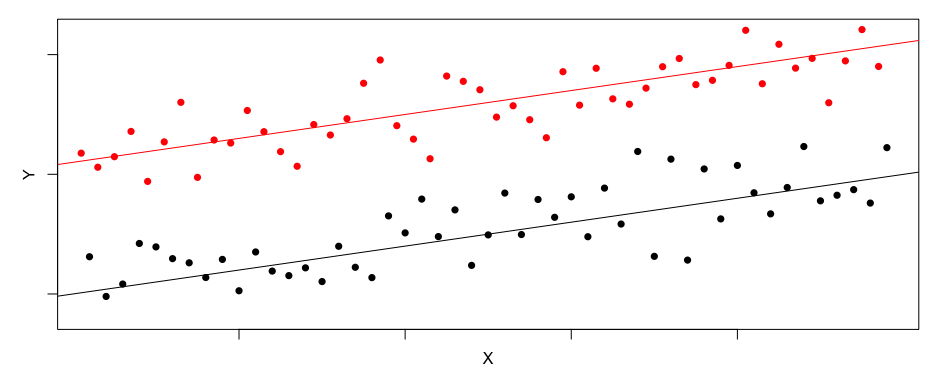
Next, plot the effect of Root size ('Root') on Fruit production ('Fruit'), separately for each level of 'Grazing'.
## Set up the axes
plot(FruitProd$Root, FruitProd$Fruit, type = "n")

## Add the data for the Grazed and Ungrazed groups
with(FruitProd, points(Root[Grazing == "Grazed"], Fruit[Grazing == "Grazed"]))
with(FruitProd, points(Root[Grazing == "Ungrazed"], Fruit[Grazing == "Ungrazed"], col = "red"))

## Add a legend
legend("bottomright", legend = c("Grazed", "Ungrazed"), pch = 1, col = c("black", "red"))
Is the range of 'Root' the same for each level of 'Grazing'?
No. "Ungrazed" ranges from about 4 to 7.5, whereas "Grazed" ranges from about 6 to 11.
Does this imply anything about the relationship between root diameter and grazing?
Yes. It suggests that root diameter and grazing are confounded explanatory variables - grazed plants have larger roots.
Could the experimental design have been changed to avoid a relationship between root diameter and grazing?
Probably not! A biologically plausible explanation of these data is that grazing directly affects root diameter - grazed plants grow larger roots.
Dependency among explanatory variables makes the ANOVA table sensitive to the order of terms in the regression model - remember you saw this when exploring the correlations of predictor variables in Practical 5.
For the present data, this is illustrated by changing the order of 'Root' and 'Grazing', and comparing ANOVA tables, as follows:
fit1 <- lm(Fruit ~ Root + Grazing, data=FruitProd)   ## Root enters the model before Grazing
anova(fit1)
fit2 <- lm(Fruit ~ Grazing + Root, data=FruitProd)  ## The order is reversed
anova(fit2)
Are the two ANOVA tables the same?
No. The only statistics not affected are the degrees of freedom. This indicates that the effect of Grazing and Roots are confounded with each other, and therefore we are unlikely to be able to pinpoint the separate effects of Grazing and Roots on fruit production.
7.6 Another example where ANCOVA can go wrong
Next we will use another example to illustrate to you the dangers of confounded predictors in ANCOVA. It's hard to imagine that anyone could design an experiment as bad as this, but let's try! We will use some data from a study of zebrafish, Danio rerio.
Aim: To evaluate whether tail depth (a measure of fish shape) can be explained by:
- fish length ('Length'; a continuous explanatory variable), and/or;
- sex (a categorical predictor variable).
The data are available the file zebrafish.csv.
zebrafish <- read.csv("zebrafish.csv", header=T)Run the following code to make a graphical display of the data, separated by 'Sex':
## Set up a blank plot of 'TailDepth' plotted against 'TotalLength'
plot(zebrafish$TotalLength, zebrafish$TailDepth, type = "n")

## Add points: Pop1 circle , Pop2 plus
with(zebrafish, points(TotalLength[Sex == "M"], TailDepth[Sex == "M"], pch = 1, col = "red"))
with(zebrafish, points(TotalLength[Sex == "F"], TailDepth[Sex == "F"], pch = 3))

## Add a legend
legend("bottomright",    ## Location of legend
legend = c("M", "F"),    ## Labels
pch = c(1, 3),           ## Plot symbols
cex = 0.8,               ## Legend magnification
col = c("red", "black")) ## Legend colours
Is the range of 'TotalLength' the same for the two sexes?
No. The vast majority of males have a body length between 20-33, whereas females are slightly longer and have body lengths between 21-37! While there is substantial overlap in 'TotalLength', females are clearly longer on average.
range(zebrafish$TotalLength[zebrafish$Sex == "F"])
Does this imply anything about the relationship between 'TotalLength' and 'Sex'?
Yes, length is highly dependent on sex.
Dependence between explanatory variables can be tested directly by regressing one against the other.
## Model the effect of the categorical variable on the continuous variable
model <- lm(TotalLength ~ Sex, data=zebrafish)
anova(model)  ## Test the effect

## Note that this is equivalent to a t-test comparing the total length of the two sexes
with(zebrafish, t.test(TotalLength[Sex == "M"], TotalLength[Sex == "F"], var.equal = TRUE))
Is there evidence of a relationship between these two explanatory variables?
Yes! The F-value is large and the P-value is very small so we reject the null hypothesis of no association.
When one explanatory variable is dependent on another explanatory variable, it is not possible to fully separate their effects upon the response variable. It causes the following problems:
- The ANOVA table depends on the order in which the explanatory variables are entered into the model, i.e., the results are ambiguous
- Estimates of partial regression slopes have inflated standard errors.
On the other hand, zero (or negligible) relationship between explanatory variables makes it easier to understand their joint effect upon the response variable.
The following code illustrates the extent of the problem when the groups are defined by 'Sex':
model1 <- lm(TailDepth ~ TotalLength + Sex, data=zebrafish) ## Model with 'TotalLength' first
model2 <- lm(TailDepth ~ Sex + TotalLength, data=zebrafish) ## Model with 'Sex' first

anova(model1)  ## Results of model1
anova(model2)  ## Results of model2
Based on these ANOVA tables, can you decide whether 'Sex' affects 'TailDepth'?
No; sex goes from being highly non-significant in model1, to highly significant in model2.
If one explanatory variable is dependent on another, then the question: "How is an explanatory variable related to the response variable?", has more than one answer.
The answer depends upon which other explanatory variables have already been accounted for in the analysis. This is unsatisfactory; we want one answer for each question (not several)!
The ambiguity exists because the two explanatory variables, 'TotalLength' depends on 'Sex': otherwise the two ANOVA tables would be identical. This problem of ambiguity (caused by strong relationships among explanatory variables) becomes unmanageable when there are many confounded explanatory variables amongst themselves to varying degrees. The interpretation of your analysis must always keep in mind if and how the explanatory variables are related to each other.
7.7 Do it on your own
Let's once again go back to the iris dataset. As you know, the iris dataset comes with R, so you will not need to load any other data into your workspace.
head(iris)
str(iris)Write out the necessary code, with comments as needed, in your script to answer the questions below:
What is the model formula (in R) to test the relationship?
If you need to, go back to section [fill in section here] for guidance
What is the null hypothesis for this analysis?
If you need to, go back to [fill in section here] for guidance
What test will you use in order to accept or reject the null hypothesis?
If you need to, go back to [fill in section here] for guidance
How will you test the assumptions of your model are met?
If you need to, go back to [fill in section here] for guidance
How will you decide if you need to transform your data?
If you need to, go back to [fill in section here] for guidance
How will you decide if the relationship of sepal and petal length depends on the species?
If you need to, go back to section [fill in section here] for guidance