Practical 10 Revisiting data descriptions and summaries - the Multivariate Approach

It takes practice to be able to do things like juggling or catching a cricket ball when fielding in slips, but with enough practice they can be come simple reflexes. Think of this practical/PBL as a training session to put you on the path to being able to interpret patterns of variation and association in data, reflexively, without having to think about it. Ultimately, these skills will allow you to readily interpret complex outcomes from analyses like multiple regression. Complete mastery of the terms and concepts covered in this practical are essential for understanding the remainder of the course. But they aren't all new! Rather, you are going to dive deep into thinking about how to describe data, using tools you have already learnt plus a couple of new ones.
There are three short lecture videos for you to watch before you come to class: 10.1, 10.2 and 10.3. The questions that follow the video assume that you have watched these lectures.
Some of the questions in these activities are nonsensical - they are just plain wrong. We'll talk about why they are wrong as a group in class.
10.1 Understanding the anatomy of the data matrix
A research group in Brisbane was interested in understanding more about the biology of garden skinks. After obtaining the appropriate animal ethics approval, they measured lizard size (weight), morphology (tail and leg lengths), how fast they run (speed) and the strength of their bite (bite force).
This data is available to you as: LizardSpeed.csv.
Import the data file and View it to address these questions:
- What is the dimensionality of this data matrix? HINT: you can ask R to confirm this for you using
dim(LizardSpeed). Note: sometimes a variable like "Individual", which here seems to be just a row number, might be excluded when thinking about the dimensionality of the data. - For how many individuals was tail length measured?
- What's the value of the 3rd object for the 2nd variable, y3,2?
- What's the value of 10th object for the 4th variable , y10,4?
- Plot the (approximate) position of object 7 in the 2-D space defined by speed and weight (y7,1 vs y7,2).
While the number of rows and columns in a data set is simple to see when we open the file (although with big datasets we might not manually count the number of rows and columns!), we can also infer the numbers of variables and objects from graphical presentation of the data. As you saw just before when you plotted lizard speed and weight, you can present the same information about the data in a graph.
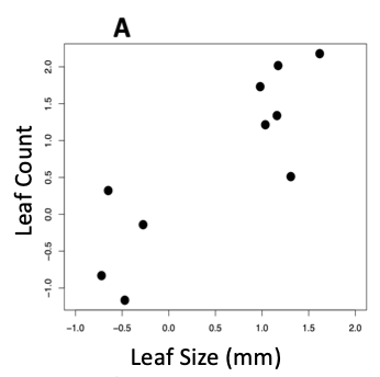
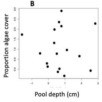
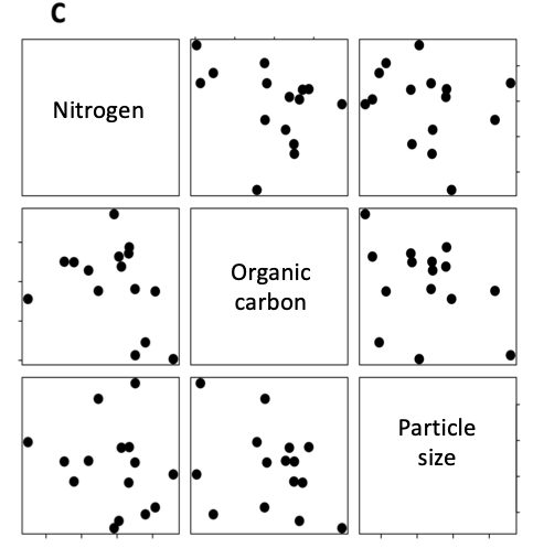
- Describe the dimensionality (n x p) of the data that was plotted for each of the experiments (A, B and C) shown below:
A. Researchers asked, "Do plants with big leaves also have many leaves?" What did the researchers measure to address this question?
B. Researchers asked, "Do deeper rockpools have more algae than shallow pools?" What did the researchers measure to address this question?
C. Researchers asked, "Do sites with sandy soils (large particles) have more carbon and nitrogen than sites with clay soils (small particles)?" What did the researchers measure to address this question?
10.2 Simple Statistics Summarising and Describing Multivariate Data
You are very familiar by now with thinking about describing data in terms of the central tendency (we've mostly focused on the mean) and spread (you have looked hard at standard deviation and standard error, and have used the sums of squares to describe spread for various predictors in linear models that you have fit).
In this activity, we want you to start thinking about how to access this information when it is presented to you in the form of a variance-covariance matrix, and to advance again your understanding of how to interpret associations between continuously distributed variables.
Plant Growth
Researchers estimated the variance in the growth rate of a particular variety (genotype) of sunflower when fertilised or not fertilized, and the covariance in growth rate between these two environments. They want to know: "Does fertilizer affect growth variability? Does growth in one environment predict growth in the other?"
##              fertilised unfertilised
## fertilised         5.19         6.08
## unfertilised 6.08 11.72- What is p of the dataset they have analysed to estimate this variance-covariance matrix? What was n?
- What is the covariance in growth rate between the two environments?
- In which environment was there greatest variance among the genotypes in their growth rate?
Dog behaviour
Researchers estimated the variance in the number of times dogs bark in an hour, and the number of sticks they return in a game of fetch, and estimated the covariance between these two variables. They were interested in understanding whether dogs that frequently bark are also good at fetch.
##             Bark Rate # of sticks
## Bark Rate       67.10        0.01
## # of sticks      0.01        0.93
What is the covariance between the two behaviours? Based on this, do you think the researchers can conclude that dogs that bark very little fetch many or few sticks?
For which behaviour did researchers estimate the greater spread in their data?
Genes changing expression
Researchers estimated the variance and covariance in the expression level of two genes involved in transcription regulation to determine if they both respond in the same way between to a drug treatment. Below is the covariance matrix they prepared for publication of their results.
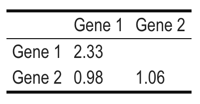
- What information have they omitted from the table? What specific value does this missing information take?
Lizard running speed
Thinking back to the data on lizard running speed that you considered in 10.1 (View(LizardSpeed)):
What information (i.e., columns and rows / variables and objects) would the researchers need to estimate the covariance between running speed and weight?
Could you calculate the covariance between speed and weight for Individual 1? Why/why not? Hint: how would you summarise n =1 data?
Estimate the variance-covariance matrix for these data:
round(cov(LizardSpeed),2)- How might you interpret the variance in "Individual"?
- Which variable has the greatest magnitude of variance?
- Which two variables have the largest covariance?
Crab carapace
## Error in knitr::include_graphics(paste0(getwd(), "/Prac10_crab.png")): Cannot find the file(s): "DataFigs/Prac10_crab.png"
A researcher measured carapace width (CW; variable 1) and claw length (CL; variable 2) of 100 Ghost crabs at each of four sites on the West Australian Coast, and calculated the variances and covariances for each site. Ultimately, they want to know if crabs with wider carapaces also have longer claws, and if this relationship differs among sites.
##       CW   CL
## CW 18.31 9.11
## CL  9.11 4.24
## CW CL
## CW 15.18 11.83
## CL 11.83 6.91## CW CL
## CW 16.88 1.45
## CL 1.45 3.37## CW CL
## CW 17.61 13.67
## CL 13.67 9.96
18. Which site has the most variance in carapace width?
19. Which site has the most variance in claw length?
20. Which site has the greatest variance in crab morphology? HINT: you will need to calculate the trace of the matrices to answer this. Trace = sum of variances (diagonal elements in variance-covariance matrix).
Site1[1,1]+Site1[2,2]
Site2[1,1]+Site2[2,2]
Site3[1,1]+Site3[2,2]
Site4[1,1]+Site4[2,2]
10.3 Scale and comparing covariances: Correlations
10.3.1 Interpreting correlation matrices
Fly phenotypic variation
## Error in knitr::include_graphics(paste0(getwd(), "/Prac10_fly.png")): Cannot find the file(s): "DataFigs/Prac10_fly.png"A researcher was interested in understanding about more about patterns of trait variation in a native Australian vinegar fly, Drosophila serrata. They measured four different variables: wing size (in mm), development time (in hours), the amount of a scent (pheromone) (in picolitres), and daily yeast consumption as as an adult (in nanograms). Each variable was measured on 20 male flies from 10 different sampling sites between Brisbane and Cairns. From this data, the researchers calculated the variance for each variable, and the covariances between variables, shown below.
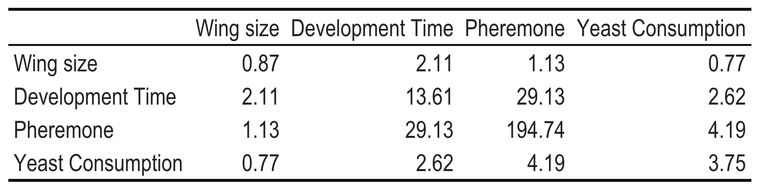
21. Which covariance do you think represents the strongest association between the two variables? What are two ways that you could assess your intuition?
We can gain some insight into the strength of an association by considering the magnitude of the covariance relative to the magnitude of the smallest variance: if they are similar, it suggests that much of the variance is shared; if the covariance is much smaller than either variance it suggests little association between that pair of variables.
It is, of course, better to be precise and calculate the correlation:
\[r = \frac {{\sigma}_{xy}}{\sqrt {{\sigma}_{xx}{\sigma}_{yy}}}\] Where \({\sigma}_{xy}\) is the covariance of \(x\) with \(y\) and \({\sigma}_{xx}\) and \({\sigma}_{yy}\) are the variances in \(x\) and \(y\), respectively (you aren't expected to memorise these formula, but seeing them can help you to understand the simple relationships between the different metrics that are used to summarise spread in the data; see also Table 2.1 in Quinn and Keough).
We can ask R to do that for us on the whole matrix, rather than calculating it for each of the six pair-wise comparisons ourselves using this equation.
Run the following code to read in their covariance matrix and estimate the correlation matrix:
FlyMatrix<-matrix(c(0.87, 2.11,1.13,0.77,
         2.11,13.61,29.13,2.62,
        1.13,29.13,194.74,4.19,
        0.77,2.62,4.19,3.75),nrow = 4 , ncol = 4)
rownames(FlyMatrix)<- c("Wing size", "Development Time", "Pheremone", "Yeast Consumption")
colnames(FlyMatrix)<- c("Wing size", "Development Time", "Pheremone", "Yeast Consumption")

round(cov2cor(FlyMatrix),2)# use base R function `cov2cor` to estimate the correlation matrix from the covariance matrix, and round to 2 decimal places for ease of interpretation.
22. How do you interpret the diagonal of this matrix?
23. Which variable pair has the strongest correlation between variables? Did this match what you expected from your inspection of the variances and covariances?
Look at the correlation matrix for the variables measured on the garden skinks by applying the cor function to the LizardSpeed data:
LizCor<-cor(LizardSpeed[,2:6])#exclude "Individual" and estimate the correlations among other variables
round(LizCor,2) # reduce number of decimal places to make it easier to read- How would you describe the association between tail length and bite force? How does that differ from you description of the association between tail length and weight?
10.3.2 Intepreting Variable associations from scatterplots
Plotting data can always give us insights into their distributions and associations.
- Describe the general characteristics of the numbers that would appear in the variance-covariance matrix for the data in each of the plots shown below. Consider specifically if there is a positive, negative or no trend in the data, and whether there a lot or a little scatter around the trend line, and so is it a strong or weak association?
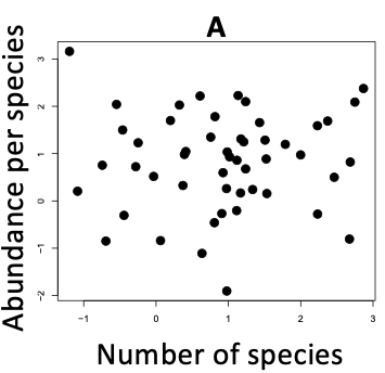
A. Researchers sampled several sites on the Great Barrier Reef and asked, "Does the number of fish species vary with species abundance?"
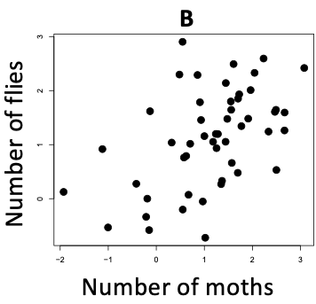
B. Using an observational study in green tree frogs, researchers asked, "do frogs that eat many moths eat relatively many or few flies?"
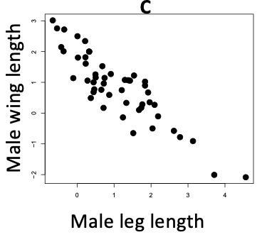
C Researchers asked, "Do leg and wing length covary in male butcher birds?"
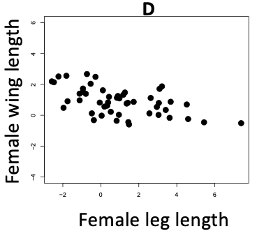
D Researchers asked, "Do leg and wing length covary in male butcher birds?"
Do you think that the strength of the correlation between wing and leg lengths differs between male and female butcher birds? What is your evidence for / against? Think very carefully about how you are interpreting these figures: remember that the correlation coefficient is not the regression slope.
http://guessthecorrelation.com/
Remember this game from Prac 5? You can play some more to train your intuition about what a strong, moderate ore weak association looks like
10.3.2.1 Drawing the association
It can also help to develop your understanding to apply this skill in the opposite way.
- Draw (as a scatterplot or as an ellipse - your tutor will demonstrate how) the pattern you would expect to see if the correlation between the number of blue flowers and the number of bees recorded for 23 gardens across Brisbane was:
- 0.76
- -0.13
- 0.48
- -0.85
- Which correlation represents the strongest association between the number of bees and the number of blue flowers?
10.3.3 Coefficient of Determination
The coefficient of determination describes how much of the variation in one variable is explained by the other. It is an identical concept to the \(R^2\) that you have encountered in regression, but it is symmetrical (in regression, we are only concerned with variance explained in our response variable). We can calculate it simply by squaring the correlation between the variables.
Considering the correlations among different five leaf traits, estimated from 11 species of plants, taken from the Reich et al. 1999 that you were introduced to in the video at 10.1 ("Generality of Leaf Trait Relationships: A Test Across Six Biomes". Ecology 80:1955-1969. We are looking at a subset of the data from the Wisconsin site.

*You can use your R coding skills to write code to calculate these (how would you change the code used to calculate the trace of the matrices in the crab example at)
28. What is the \(r^2\) of A~mass and A~area?
29. What is the \(r^2\) of SLA and Gs?
30. Which two variables have the smallest \(r^2\), and what do you think that means? What about the largest?